Online State Estimation Using Identified Nonlinear Models
This example describes how to generate the state-transition and measurement functions for online state and output estimation using nonlinear system identification techniques.
System Identification Toolbox™ provides several recursive algorithms for state estimation such as Kalman Filter, Extended Kalman Filter (EKF), Unscented Kalman Filter (UKF), and Particle Filter (PF). Use of a state estimator requires specification of state and measurement dynamics:
How the system advances the states, represented by the state-transition equation, where is the state value at the time step ; the functioncan accept additional input arguments to accommodate any dependency on exogenous inputs and the time instant.
How the system computes the output or measurement as a function of and possibly some additional inputs;
In addition, you are required to provide the covariance values of the various disturbances affecting the state and measurement dynamics.
This example shows how you can generate the required state-transition and measurement equations by using nonlinear (black-box or grey-box) identification techniques. Four different modeling techniques are explored - Nonlinear ARX, Hammerstein-Wiener, Neural State Space and Nonlinear Grey Box.

This example describes:
How to extract, and separate out, the state-transition and measurement functions from identified nonlinear models of various types.
How to separate out noise dynamics in case the nonlinear model uses a nontrivial (that is, not an Output-Error structure) disturbance component; this is true only for the Nonlinear ARX models.
How to extend the nonlinear models of Output-Error structure in order to prescribe the state/process noise covariance required by the state estimators such as EKF.
Definition of an Output-Error Model Structure
A generic discrete-time dynamic model in the System Identification Toolbox has the following representation:
where the function relates the past values of the output , the current/past values of the input , and the disturbances current/past values to the current value of the output. In the linear case, this can be written as a stochastic relationship using additive noise:
where , are linear filters described by rational functions. When the noise filter , the model is called an Output-Error model. This is because when =1, the governing equation simplifies to:
Here, the output at time is not affected by errors at previous time instants. In state-space form, this translates to a model of the form:
This is a system with no process noise. A state estimator based on this model cannot correct the state predictions using current output measurements. Hence an Output-Error model needs to extended in some way to extract the process noise information.
Most nonlinear models in the System Identification Toolbox are of Output-Error structure. The only exception is Nonlinear ARX models, where the model structure is:
where are measured (noise-corrupted) outputs values. The influence of past errors can be seen more clearly by writing the equation in terms of the true (noise free) output , so that :
Example System: An Industrial Robot Arm
Consider a robot arm is described by a nonlinear three-mass flexible model. The input to the robot is the applied torque generated by the electrical motor, and the resulting angular velocity of the motor is the measured output.
It is possible to derive the equations of motion for this system. For example a nonlinear state-space description of this system uses 5 states. For more information on this system, see the example titled "Modeling an Industrial Robot Arm".

This system is excited with inputs of different profiles and the resulting angular velocity of the motor recorded. A periodic excitation signal with approximately 10 seconds duration was employed to generate a reference speed for the controller. The chosen sampling frequency was 2 kHz (sample time, Ts = 0.0005 seconds). For estimation (training) data, a multisine input signal with a flat amplitude spectrum in the frequency interval 1-40 Hz with a peak value of 16 rad/s was used. The multisine signal is superimposed on a filtered square wave with amplitude 20 rad/s and cut-off frequency 1 Hz. For validation data, a multisine input signal containing frequencies 0.1, 0.3, and 0.5 Hz was used, with peak value 40 rad/s.
Both datasets are downsampled 10 times for the purposes of the current example.
load robotarmdata.mat
% Prepare estimation data
eData = iddata(ye,ue,5e-4,'InputName','Torque','OutputName','Angular Velocity','Tstart',0);
eData = idresamp(eData,[1 10]);
eData.Name = 'estimatipen_systemn data'
eData =
Time domain data set with 1984 samples.
Sample time: 0.005 seconds
Name: estimatipen_systemn data

Outputs                Unit (if specified)
   Angular Velocity

Inputs                 Unit (if specified)
   Torque

Data Properties
% Prepare validation data
vData = iddata(yv3,uv3,5e-4,'InputName','Torque','OutputName','Angular Velocity','Tstart',0);
vData = idresamp(vData,[1 10]);
vData.Name = 'validation data';
idplot(eData, vData)
legend show

Nonlinear Black Box Model
Suppose you have prior knowledge that the underlying process is nonlinear (or that the linear black box model does not provide a good result), but you do not have detailed knowledge of the underlying physics. In that case you can identify nonlinear black-box models of different structures. Then use the identified models to build up the state estimators.
Nonlinear ARX Model
A nonlinear ARX model is a discrete-time model that has the following structure:
That is, the output at time is computed as a nonlinear function of past outputs and present and past inputs. At any time step the disturbance gets added to the output. All future values would typically contain the effect of this disturbance since the past outputs are used to compute the future ones. In a sense, the effect of disturbances accumulate as time progresses. As a result, long-term predictions are usually harder with these models especially if they have been trained in open loop (for example, by using Focus = 'prediction' with the nlarx command).
IDNLARX Model States
The states of this model are defined as the lagged input/output variables. So a nonlinear ARX model using the equation:
can be expressed in state-space form by using the state variables:
leading to the following state-space representation:
Define . Then in the matrix form you have the following representation:
where is a constant matrix, and the vector function . Note that in this form, the process and measurement noises are correlated.
Identification of Wavelet Network Based Nonlinear ARX Model
Identify a Nonlinear ARX model for the robot arm data.
vars = {'Angular Velocity','Torque'};
L = linearRegressor(vars,1:2:8);
P = polynomialRegressor(vars,1:2:8,3);
opt = nlarxOptions(SearchMethod='gna',Focus='simulation');
nlarx1 = nlarx(eData, [L;P], idWaveletNetwork(3), opt)
nlarx1 = Nonlinear ARX model with 1 output and 1 input Inputs: Torque Outputs: Angular Velocity Regressors: 1. Linear regressors in variables Angular Velocity, Torque 2. Order 3 regressors in variables Angular Velocity, Torque List of all regressors Output function: Wavelet network with 3 units Sample time: 0.005 seconds Status: Estimated using NLARX on time domain data "estimatipen_systemn data". Fit to estimation data: 78.18% (simulation focus) FPE: 6.334, MSE: 20.65 Model Properties
% Perform 10 step ahead prediction for the output data in the validation dataset.
compare(vData, nlarx1, 10);
Using the Model in the Extended Kalman Filter (EKF) Block
In order to use this model in the EKF block, you need to specify the state-transition and measurement functions as Simulink functions. For the current example, these are implemented using MATLAB Function Blocks. The nlarxPredictFcn function performs the core computation; this function is called by the MATLAB Function blocks implementing the state transition and measurement updates.
type nlarxPredictFcnfunction [y,xnext] = nlarxPredictFcn(x,u)
% Predict the states and output of a nonlinear ARX model.
% The identified model ("nlarx1") is assumed to be available in the MATLAB base workspace.
% Copyright 2022 The MathWorks, Inc.
sys = evalin('base','nlarx1');
% Step 1: Compute model regressors as a function of states. Use GETERG to see the list of
% regressors. Regressors are non-tunable, static functions of model states and inputs.
I = [1 3 5 7 8 10 12 14];
R = [x(I,:); x(I,:).^3].';
% Step 2: Map the regressors to the model output. This is required since x1(t+1) = y(t) for this
% model. Note that output y is a static function (represented by the wavelet network) of the model's
% regressors (R).
N = sys.Normalization;
NL = sys.OutputFcn;
R = (R-N.RegressorCenter)./N.RegressorScale;
y = evaluate(NL, R);
y = (y.*N.OutputScale + N.OutputCenter).';
if nargout>1
% Compose the output xnext := x(t+1)
xnext = x; % initialization
xnext(1,:) = y;
xnext(2:7,:) = x(1:6,:);
xnext(8,:) = u;
xnext(9:14,:) = xnext(8:13,:);
end
The state estimation scenario based on the identified model (nlarx1) is implemented in the Simulink model StateEstimation_Using_NonlinearARX.slx. The scenario considered is 10-step ahead prediction realized by enabling the multi-rate operation; the measurements are used for correction of the state estimates only once for every 10 successive predictions.
% Prepare some data for the EKF Block
NV = nlarx1.NoiseVariance; % measurement noise variance
K = zeros(14,1); % (there are 14 states)
K(1) = 1;
StateNoiseCovariance = K*NV*K';
Ts = nlarx1.Ts;  % prediction time interval
Ts2 = 10*Ts;     % correction time interval

open_system('StateEstimation_Using_NonlinearARX')

Using the Model in the Unscented Kalman Filter (UKF) Block
The UKF block is configured in the same manner as the EKF block. The Simulink functions stateTransitionFcn and measurementFcn in the model StateEstimation_Using_NonlinearARX.slx are used by both the EKF and UKF blocks.
Using the Model in the Particle Filter (PF) Block
For the Particle Filter block, you need to specify the transition function for the particles and the value of the measurement likelihood as a probability distribution.
NumParticles = 1000; % number of particles used by the Particle filter
10 Step Ahead State Estimation Results
sim('StateEstimation_Using_NonlinearARX');


For this example, the three state estimators perform similarly. Note that the system output is same as the first state value. The filters underestimate the outputs at certain regions of rapid change. This observation is consistent with the direct 10-steap ahead prediction result shown in the compare plot.
Hammerstein Wiener Model
Another popular type of nonlinear dynamic model is a Hammerstein-Wiener model. It connects static nonlinear functions in series with a linear transfer function. The states of this model are the states of its linear block.
% Estimate a model that uses piecewise linear functions for its input and output nonlinearities
nlhw1 = nlhw(eData,[7 7 1])
nlhw1 = Hammerstein-Wiener model with 1 output and 1 input Linear transfer function corresponding to the orders nb = 7, nf = 7, nk = 1 Input nonlinearity: Piecewise linear with 10 breakpoints Output nonlinearity: Piecewise linear with 10 breakpoints Sample time: 0.005 seconds Status: Estimated using NLHW on time domain data "estimatipen_systemn data". Fit to estimation data: 87.98% FPE: 6.637, MSE: 6.266 Model Properties
compare(vData, nlhw1) % validate the model quality on an independent dataset
A Hammerstein Wiener model is an output-error model; there is no process noise. However, one can consider extending the identified model by prescribing process noise of non-zero covariance (covariance value determination would require a separate analysis). For this example, this extension is not explored.
uNL = nlhw1.InputNonlinearity;
yNL = nlhw1.OutputNonlinearity;
linTF = nlhw1.LinearModel;
[A,B,C,D] = ssdata(linTF);
Ts = nlhw1.Ts;

For using this model for state estimation, you can use the intermediate signal w(t) as the input signal since the I/O nonlinearities do not contain any states.
t = vData.SamplingInstants; % the time vector for the validation data
u = vData.InputData; % the input signal u(t)
w = evaluate(uNL, u); % the output of the "Input Nonlinearity f" block w(t)
The model states can be obtained by simulating the linear block using the signal w(t) and any prescribed initial conditions. For example:
[~,~,x] = sim(nlhw1, w);
plot(t,x)
xlabel('Time (seconds)')
ylabel('States (X)')

shows the state trajectories generated for zero initial conditions.
Since there is no process noise, there is no correction step required in the state predictors. The entire state prediction exercise is same as a pure simulation. The state estimators such as EKF are required only when there is an opportunity to correct the estimates using the measurements. This is explored more in the context of state-space models.
Nonlinear State Space Models
Neural State Space Model
A neural state space model is a continuous- or discrete-time nonlinear model where you specify the state transition and measurement functions as multi-layer feedforward neural networks. This modeling technique requires Deep Learning Toolbox™. Neural state space models are output-error models - they assume the states are not affected by process noise.
Training a neural state space model requires measurements of the states as well as the outputs. Assume that the state definitions are not available. Hence define states in terms of lagged inputs and outputs. You can generate data for the lagged variables by using the getreg command that is called on a template Nonlinear ARX model that uses the regressors defined as the lagged variables.
eData2 = idresamp(eData,[1 2]); % reduce data for quicker results

% normalize the data
eM = mean([eData2.OutputData,eData2.InputData]);
eSD = std([eData2.OutputData,eData2.InputData]);
eData2.OutputData = (eData2.OutputData-eM(1))/eSD(1);
eData2.InputData = (eData2.InputData-eM(2))/eSD(2);

Ts = eData2.Ts;
vars = {'Angular Velocity','Torque'};
nx = 7;
L = linearRegressor(vars,1:nx);
n0 = idnlarx(vars(1),vars(2),L,'Ts',Ts);
% View the state variables
States = getreg(n0); % there are 8 states
disp(strjoin(States,'\n'))
Angular Velocity(t-1)
Angular Velocity(t-2)
Angular Velocity(t-3)
Angular Velocity(t-4)
Angular Velocity(t-5)
Angular Velocity(t-6)
Angular Velocity(t-7)
Torque(t-1)
Torque(t-2)
Torque(t-3)
Torque(t-4)
Torque(t-5)
Torque(t-6)
Torque(t-7)
% get training data corresponding to these states
XData = getreg(n0, eData2);

% convert data into an iddata object; add the actual output (Angular Velocity(t)) as the last
% output signal
ymeas = eData2.OutputData;
xmeas = XData{:,:};
XYData = iddata([xmeas,ymeas],eData2.InputData,...
   'OutputName',[States; vars(1)],'InputName',vars(2),'Ts',Ts,'Tstart',0);

% Discard first 4 samples that contain effects of unknown initial conditions
XYData = XYData(nx+1:end);
Create a Neural State Space model that uses 14 states and one input. Since the states are considered measured, the model has 15 outputs, one corresponding to each state, plus the actual output.
nss = idNeuralStateSpace(numel(States),NumInputs=1,NumOutputs=numel(States)+1,Ts=Ts);
Model the state-transition function as a 1 hidden layer network using sigmoid activation layer.
rng(5) % for reproducibility
nss.StateNetwork = createMLPNetwork(nss,'state', ...
    LayerSizes=numel(States), ...
    Activations="sigmoid", ...
    WeightsInitializer="glorot", ...
    BiasInitializer="zeros");
summary(nss.StateNetwork)
   Initialized: true

   Number of learnables: 434

   Inputs:
      1   'x[k]'   14 features
      2   'u[k]'   1 features
The first 14 outputs are the states themselves Hence nss.OutputNetwork(1) is a trivial network representing the equation . The 15th output of this model represents the true measured output . For this output, create a separate, single hidden layer feedforward network using tanh activation layer.
nss.OutputNetwork(2) = createMLPNetwork(nss,'output', ...
    LayerSizes=1, ...
    Activations="sigmoid", ...
    WeightsInitializer="ones", ...
    BiasInitializer="zeros");
summary(nss.OutputNetwork(2))
   Initialized: true

   Number of learnables: 17

   Inputs:
      1   'x[k]'   14 features
      2   'u[k]'   1 features
Prepare training data by splitting it into 4 overlapping segments.
NumBatches = 4;
Ns = size(XYData,1);
Nsb = 300;
Data = cell(1,NumBatches);
pt = 0;
for i = 1:NumBatches
   if pt+Nsb<=Ns
      Data{i} = XYData(pt+(1:Nsb));
   else
      Data{i} = XYData(pt+1:end);
   end
   Data{i}.Tstart = 0;
   pt = pt + Nsb-20; % 20 sample overlap
end
Data = merge(Data{:});
Prepare training options. Choose ADAM Solver and increase the learning rate to 0.002. Also set other options such as maximum number of epochs to run and the frequency of validation plot update.
opt = nssTrainingOptions('adam');
opt.MaxEpochs = 1500;
opt.MiniBatchSize = Nsb;
opt.LearnRate = 0.02;
Train the model, where you use the last experiment in Data for in-estimation cross validation.
tic
nss = nlssest(Data,nss,opt,UseLastExperimentForValidation=true)


Generating estimation report...done.

nss =

Discrete-time Neural State-Space Model with 15 outputs, 14 states, and 1 inputs
     x(t+1) = f(x(t),u(t))
     y_1(t) = x(t) + e_1(t)
     y_2(t) = g(x(t),u(t)) + e_2(t)
       y(t) = [y_1(t); y_2(t)]

f(.) network:
  Deep network with 1 fully connected, hidden layers
  Activation function: sigmoid
g(.) network:
  Deep network with 1 fully connected, hidden layers
  Activation function: sigmoid

Inputs: Torque
Outputs: Angular Velocity(t-1), Angular Velocity(t-2), Angular Velocity(t-3), Angular Velocity(t-4), Angular Velocity(t-5), Angular Velocity(t-6), Angular Velocity(t-7), Torque(t-1), Torque(t-2), Torque(t-3), Torque(t-4), Torque(t-5), Torque(t-6), Torque(t-7), Angular Velocity
States: x1, x2, x3, x4, x5, x6, x7, x8, x9, x10, x11, x12, x13, x14
Sample time: 0.01 seconds

Status:
Estimated using NLSSEST on time domain data "Data".
Fit to estimation data: [61.38 54.91 54.84 54.78 55.53 58.27 56.77 37.44 12.33 4.976....%
FPE: 2.747e-15, MSE: [6.416 6.424 6.04 5.826]

Model Properties
toc
Elapsed time is 1196.284955 seconds.
[yp,fit] = compare(XYData, nss);
plot(XYData(:,end,[]),yp(:,end,[]))
legend('measured',['model (',num2str(fit(end)),'%)'])

This estimation takes a long time. For reference, the results are available in the data file IdentifiedNeuralSSModel.mat.
Just like the Hammerstein-Wiener model, a Neural State Space model is an Output Error model. This means that there is no process noise considered as part of the state transition. However, the identified model can be extended post-estimation with a process noise component.
% Simulate the state trajectory
[~,~,Xp] = sim(nss,XYData);
% Fetch measured values of the states
X_measured = XYData.OutputData(:,1:end-1);
% Compute covariance of dX := Xp-X_measured
dX = Xp-X_measured;
XCov = cov(dX);
NV = nss.NoiseVariance;
Xsd = chol(XCov);
NVc = chol(NV);
NumParticles = 1000;
x0 = X_measured(1,:)'
x0 = 14×1

    -1.6494
    -1.0918
    -1.3285
    -0.5497
    -0.5271
    -1.0293
    -0.8808
    -1.1322
    -0.3761
    -0.5067
    -1.8215
     0.7533
    -0.7358
    -1.6756
      ⋮
Use the generateMATLABFunction command to generate MATLAB functions that implement the state-transition and the measurement functions. The functions are generated as M files. An accompanying MAT file is also generated and it must be present together with the M files for the interface to work properly in downstream applications.
Run the following command in a folder with write privileges to generate the Jacobian files nssStateFcn.m, nssMeasurementFcn.m, and the accompanying files.
generateMATLABFunction(nss, "nssStateFcn", "nssMeasurementFcnOutput15");
The generated functions - nssStateFcn and nssMeasurementFcnOutput15 use persistent variables which are not allowed to be used inside MATLAB System blocks (the MATLAB System blocks are used to implement the predictor and corrector functions). Hence we modify these functions, post generation, to remove the use of the persistent variables. The modified functions are called nssStateFcn_2 and nssMeasurementFcnOutput15_2 respectively.
type nssStateFcn_2function x1 = nssStateFcn_2(x,u) %% state function of neural state space system % created by modifying the auto-generated function nssStateFcn %# codegen MATname = 'nssStateFcnData'; StateNetwork = coder.load(MATname); out = [x;u]; % hidden layer #1 out = StateNetwork.fc1.Weights*out + StateNetwork.fc1.Bias; out = deep.internal.coder.sigmoid(out); % output layer dx = StateNetwork.output.Weights*out + StateNetwork.output.Bias; x1 = x + dx;
type nssMeasurementFcnOutput15_2function y = nssMeasurementFcnOutput15_2(x,u) %% output function of neural state space system % created by modifying the auto-generated function to remove the use of persistent variables %# codegen MATname = 'nssMeasurementFcnOutput15Data'; OutputNetwork = coder.load(MATname); out = x; % hidden layer #1 out = OutputNetwork.fc1.Weights*out + OutputNetwork.fc1.Bias; out = deep.internal.coder.sigmoid(out); % output layer y = OutputNetwork.output.Weights*out + OutputNetwork.output.Bias;
Note that the measurement function file represents only the extra outputs (output numbers nx+1:ny). This is output signal number 15 in XYData. For use in EKF/UKF filters, we need a measurement function that describes all the outputs. Hence we wrap the nssMeasurementFcnOutput15 function in another function called nssMeasurementFcnAllOutputs which appends the model states as its first 14 outputs.
type nssMeasurementFcnAllOutputsfunction y = nssMeasurementFcnAllOutputs(x,u) %% output function of neural state space system % all outputs %# codegen y15 = nssMeasurementFcnOutput15_2(x,u); y = [x; y15];
The state-transition function (nssStateFcn.m) and the measurement function (nssMeasurementFcnAllOutputs.m) along with the process noise covariance (XCov) and measurement noise covariance (NV) can be used to set up online state estimators. This is implemented in StateEstimation_Using_NeuralSS.slx.
Ts = nss.Ts;
Ts2 = Ts*10; % correction time interval
open_system('StateEstimation_Using_NeuralSS')


The 10-step ahead prediction results are shown in the 3 scope plots (one for each type of filter), obtained for XYData.
sim('StateEstimation_Using_NeuralSS');


Nonlinear Grey Box Model
Finally, we explore the modeling approach that requires the maximum amount of physical knowledge regarding the dynamics. This results in a 5th order nonlinear differential equation. In state-space form these equations are:
where:
are the moments of inertia of the motor, the gear-box and the arm structure, respectively
are damping parameters
is the stiffness of the arm structure.
The gear-box friction torque , where and are the viscous and the Coulomb friction coefficients, and are coefficients for reflecting the Stribeck effect, and is a parameter used to obtain a smooth transition from negative to positive velocities of .
The torque of the spring , where are stiffness parameters of the gear-box spring.
The equations can be described by a Nonlinear Grey Box model (the idnlgrey object). The model structure for a nonlinear grey-box model is:
where denotes the set of parameters used in the functions . The identification task is to estimate in order to minimize the difference between the simulated response of the model and its measured value. The procedure is similar to the one described above for the linear grey box case - the main task is to write an ODE file that returns the state derivatives , and output as a function of and the parameters. This exercise is the focus of the example "Modeling an Industrial Robot Arm". For current purposes, load the estimation results from this example.
load RobotArmNonlinearGreyBoxModel nlgr
nlgr.Name = 'Original Model (no process noise)';
nlgr
nlgr =

Continuous-time nonlinear grey-box model defined by 'robotarm_c' (MEX-file):

   dx/dt = F(t, x(t), u(t), p1, ..., p13)
    y(t) = H(t, x(t), u(t), p1, ..., p13) + e(t)

 with 1 input(s), 5 state(s), 1 output(s), and 7 free parameter(s) (out of 13).

Name: Original Model (no process noise)

Status:
Estimated using Solver: ode45; Search: lsqnonlin on time domain data "estimation data".
Fit to estimation data: 85.52%
FPE: 9.184, MSE: 9.092

Model Properties
compare(vData, nlgr)

Similar to the linear case, you can embed the identified nonlinear grey box model into a more general stochastic framework by adding process noise to the equations for , that is, pose , where is the process noise gain matrix. However, there is no direct way to compute the value of under the nonlinear grey-box estimation framework. This is because the Nonlinear Grey Box methodology only handles Output-Error models, that is, it does not consider the influence of process noise.
An option is to pose a simple extension , where is the output prediction error. This is similar to the innovations form of the linear state-space model, where
For prediction of model output, the nonlinear predictor therefore takes the form:
In order to make this extension, add as a free parameter (5x1 vector) to the model nlgr. Also, the ODE function needs to compute . Replace the original ODE function employed by nlgr (robot_c) with a new one called robotARMNonlinearODE. For this, pass a gridded interpolator as a function argument.
type robotARMNonlinearODEfunction [dx, y] = robotARMNonlinearODE(t, x, u, Fv, Fc, Fcs, alpha, beta, J, am, ...
ag, kg1, kg3, dg, ka, da, K, Interpolator)
%robotARMNonlinearODE A physically parameterized robot arm.
% t: time instant (seconds)
% x: state value at time t (5 x 1 vector)
% u: input at time t (scalar)
% Fv, Fc, Fcs, alpha, beta, J, am, ag, kg1, kg3, dg, ka, da: parameters related to the model
% dynamics
% K: process noise gain matrix (free parameter)
% Interpolator: griddedInterpolant object to fetch measured output at a time t
% Copyright 2005-2022 The MathWorks, Inc.
% Output equation.
y = x(3); % Rotational velocity of the motor.
% Intermediate quantities (gear box).
tauf = Fv*x(3)+(Fc+Fcs/cosh(alpha*x(3)))*tanh(beta*x(3)); % Gear friction torque.
taus = kg1*x(1)+kg3*x(1)^3; % Spring torque.
% State equations.
dx = [x(3)-x(4); ... % Rotational velocity difference between the motor and the gear-box.
x(4)-x(5); ... % Rotational velocity difference between the gear-box and the arm.
1/(J*am)*(-taus-dg*(x(3)-x(4))-tauf+u); ... % Rotational velocity of the motor.
1/(J*ag)*(taus+dg*(x(3)-x(4))-ka*x(2)-da*(x(4)-x(5))); ... % Rotational velocity after the gear-box.
1/(J*(1-am-ag))*(ka*x(2)+da*(x(4)-x(5))) ... % Rotational velocity of the robot arm.
];
ym = Interpolator{1}(t);
dx = dx + K*(ym-y);
The last line of code adds a correction term to the state derivatives based on the output prediction error. In order to compute the measured output value at a given time instant, we can simply interpolate the values in eData.OutputData. To enable this, we pass a gridded interpolant as an extra input argument to the ODE function (see the last input argument "Interpolator"). When setting up the nonlinear grey-box model (idnlgrey object), you can specify any extra arguments to the ODE function using the FileArgument property.
% Change the ODE function of nlgr from "motor_c" to "robotARMNonlinearODE". robotARMNonlinearODE is
% mostly identical to motor_c except for the addition of the correction to dx induced by the process
% noise.
PredictorModel = nlgr;
PredictorModel.Name = 'Predictor form';
PredictorModel.FileName = 'robotARMNonlinearODE';

% Create a new parameter to represent the process noise gain K
% Set 0 as initial guess for K entries
NoiseGain = struct('Name','K','Unit','','Value',zeros(5,1),...
   'Minimum',-Inf(5,1),'Maximum',Inf(5,1),'Fixed',false(5,1));

% Add this parameter to the model
PredictorModel.Parameters(end+1) = NoiseGain;

% Create a linear interpolator
t = eData.SamplingInstants;
y = eData.OutputData; % measured output
Interpolator = griddedInterpolant(t,y);
Interpolator.ExtrapolationMethod = 'nearest';
PredictorModel.FileArgument = {Interpolator};
Perform parameter estimation, Because of the process noise correction, the estimation is implicitly minimizing the 1-step ahead prediction error (rather than the default behavior which is to minimize the simulation error)
opt = nlgreyestOptions('Display', 'on','SearchMethod','lm');
opt.SearchOptions.MaxIterations = 20;
opt.EstimateCovariance = false; % to speed up estimation
% Keep the parameter estimates close to their initial guesses. This is because we already have a
% good guess of their values from previous estimation as carried out in the example "Modeling an
% Industrial Robot Arm"
opt.Regularization.Lambda = .1;
opt.Regularization.Nominal = 'model';

% Estimate the model parameters
PredictorModel = nlgreyest(eData, PredictorModel, opt)
PredictorModel =

Continuous-time nonlinear grey-box model defined by 'robotARMNonlinearODE' (MATLAB file):

   dx/dt = F(t, x(t), u(t), p1, ..., p14, FileArgument)
    y(t) = H(t, x(t), u(t), p1, ..., p14, FileArgument) + e(t)

 with 1 input(s), 5 state(s), 1 output(s), and 12 free parameter(s) (out of 18).

Name: Predictor form

Status:
Estimated using Solver: ode45; Search: lm on time domain data "estimatipen_systemn data".
Fit to estimation data: 90.87%
FPE: 3.674, MSE: 3.618

Model Properties
compare(eData, nlgr, PredictorModel)

% Fetch the computed process noise gain matrix
K = PredictorModel.Parameters(end).Value
K = 5×1
0.3661
-0.4355
44.7611
-7.1629
-0.3052
% Fetch the output noise variance
NV = PredictorModel.NoiseVariance
NV = 0.0182
Validate the model.
% Check 1-step ahead prediction quality on validation dataset
tv = vData.SamplingInstants;
yv = vData.OutputData; % measured output
Interpolator2 = griddedInterpolant(tv,yv);
Interpolator2.ExtrapolationMethod = 'nearest';
PredictorModel.FileArgument = {Interpolator2};
compare(vData, nlgr, PredictorModel)

As seen from both the comparisons to the training data (eData) as well as the validation data (vData), the correction applied to the state-transition using the noise gain K has a beneficial effect on 1-step ahead predictions. Note that the original model (nlgr) has no process noise component. Hence for this model, 1-step ahead prediction is same as pure simulation.
You now have all the information available to implement nonlinear state estimators. Use the functions , as implemented in robotARMNonlinearODE to specify the state transition and measurement functions for the filters. The process noise is zero-mean Gaussian with a variance equal to , where =NV is the measurement covariance.
10-Step Ahead Prediction
Compute 10-step ahead prediction of the vData output using EKF, UKF, and PF state estimators based on PredictorModel.
% Gather block data
Ts = eData.Ts; % prediction interval
Ts2 = 10*Ts; % correction interval
% Parameter variables for use in the filter blocks
[Fv, Fc, Fcs, alpha, beta, J, am, ag, kg1, kg3, dg, ka, da, K] = deal(PredictorModel.Parameters.Value);
NumParticles = 1000; % number of particles used by the Particle filter

open_system('StateEstimation_Using_NonlinearGreyBox')
The Simulink model is set up to use a fixed step discrete solver with a fixed-step size of Ts/100 = 50 ms. The state transition equation used by the filters is implemented in the nlgreyPredictFcn function. This model is setup in a manner very similar to the one for Nonlinear ARX model based state prediction (see StateEstimation_Using_NonlinearARX.slx)
type nlgreyPredictFcnfunction xnext = nlgreyPredictFcn(x,u,Fv, Fc, Fcs, alpha, beta, J, am, ...
ag, kg1, kg3, dg, ka, da, Ts)
% Predict the state update for the nonlinear grey box model of robot arm.
% State transition function for the UKF/EKF block.
% Ts: data sample time. The model has been configured to use a fixed step size of Ts/100.
% Copyright 2022 The MathWorks, Inc.
% Euler integration of continuous-time dynamics x'=f(x) with sample time dt
xnext = x;
for i = 1:size(x,2)
xnext(:,i) = x(:,i) + continuousTimeDerivative(x(:,i),u,...
Fv,Fc,Fcs,alpha,beta,J,am,ag,kg1,kg3,dg,ka,da)*Ts/100;
end
end
%---------------------------------------------------------------------------------------------------
function dx = continuousTimeDerivative(x,u,Fv, Fc, Fcs, alpha, beta, J, am, ...
ag, kg1, kg3, dg, ka, da)
% Robot arm state derivatives.
tauf = Fv*x(3)+(Fc+Fcs/cosh(alpha*x(3)))*tanh(beta*x(3)); % Gear friction torque.
taus = kg1*x(1)+kg3*x(1)^3; % Spring torque.
% State equations.
dx = [x(3)-x(4); ... % Rotational velocity difference between the motor and the gear-box.
x(4)-x(5); ... % Rotational velocity difference between the gear-box and the arm.
1/(J*am)*(-taus-dg*(x(3)-x(4))-tauf+u); ... % Rotational velocity of the motor.
1/(J*ag)*(taus+dg*(x(3)-x(4))-ka*x(2)-da*(x(4)-x(5))); ... % Rotational velocity after the gear-box.
1/(J*(1-am-ag))*(ka*x(2)+da*(x(4)-x(5))) ... % Rotational velocity of the robot arm.
];
end
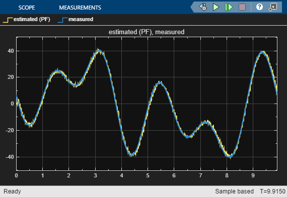
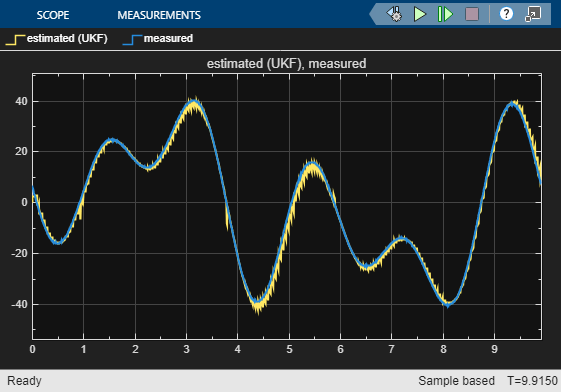
The 10-step ahead prediction results are shown in the 3 scope plots (one for each type of filter)
sim('StateEstimation_Using_NonlinearGreyBox');