Georeference an Image to an Orthotile Base Layer
This example shows how to register an image to an Earth-based coordinate reference system (CRS) and create a new georeferenced image.
The steps of the example include:
Read orthophoto base tiles that are georeferenced to map coordinates.
Read an aerial photograph that is not georeferenced.
Register the aerial photograph to map coordinates.
Use the registration to apply a geometric transformation to the aerial photograph.
Display the aerial photograph in map coordinates.
Overlay a vector layer of road data.
All georeferenced data in the example uses the Massachusetts State Plane projected CRS. The projected CRS defines the map coordinates. The reference ellipsoid underlying the projected CRS is the North American Datum of 1983 in units of meters.
Read and Display Orthophoto Base Tiles
Read two orthophoto base tiles for West Concord, Massachusetts into the workspace. Create reference objects for the orthophotos by reading their world files.
[baseImage1,cmap1] = imread("concord_ortho_w.tif");
[baseImage2,cmap2] = imread("concord_ortho_e.tif");

R1 = worldfileread("concord_ortho_w.tfw","planar",size(baseImage1));
R2 = worldfileread("concord_ortho_e.tfw","planar",size(baseImage2));
Merge the tiles into one image.
[baseImage,R] = mergetiles(baseImage1,R1,baseImage2,R2);
Verify that the colormaps for the images are equal.
isequal(cmap1,cmap2)
ans = logical
   1
Generalize the name of the colormap variable cmap1 to cmap.
cmap = cmap1;
Display the merged image on a map. Add a title, subtitle, and axes labels.
figure
mapshow(baseImage,cmap,R)

title("West Concord, Massachusetts")
subtitle("Massachusetts State Plane")

xlabel("Easting (meters)")
ylabel("Northing (meters)")

Store the current axes in a variable for future use.
ax1 = gca;
Read and Display Aerial Photograph
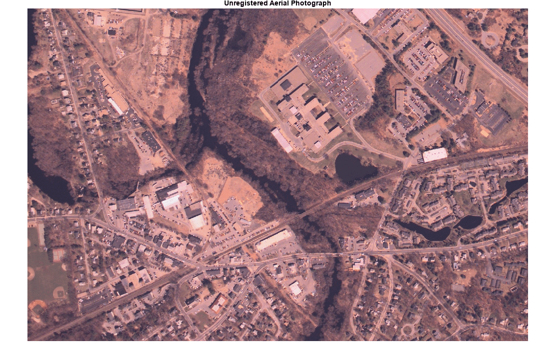
Read and display an aerial photograph of West Concord, Massachusetts. The orthophoto base tiles cover the extent of the photograph.
inputImage = imread("concord_aerial_sw.jpg");

figure
imshow(inputImage)
title("Unregistered Aerial Photograph")
Register Aerial Photograph to Map Coordinates
Register the aerial photograph to map coordinates by selecting control point pairs that relate the aerial photograph to the orthophoto base layer. Control points are landmarks that you can identify in both images, such as road intersections or natural features.
The merged orthophoto image is an indexed image. Prepare to select control points by converting the indexed image to a grayscale image.
baseGray = im2uint8(ind2gray(baseImage,cmap));
Load six preselected control point pairs from the file cpstruct.mat.
load cpstruct.mat Optionally, edit the preselected points or add additional points by using the Control Point Selection tool. Before opening the tool, downsample the images by a factor of 2. Save the control points by selecting the File menu and clicking Save Points to Workspace. Save the points by overwriting the cpstruct variable.
n = 2;
% inputImageDownsample = inputImage(1:n:end,1:n:end,1);
% baseGrayDownsample = baseGray(1:n:end,1:n:end);
% cpselect(inputImageDownsample,baseGrayDownsample)
Apply Geometric Transformation to Aerial Photograph
Extract the control point pairs from the control point structure. Account for the downsampling.
[input,base] = cpstruct2pairs(cpstruct);
input = n*input - 1;
base = n*base - 1;
Convert the coordinates of the base image to map (State Plane) coordinates.
[x,y] = intrinsicToWorld(R,base(:,1),base(:,2));
spatial = [x y];
Create a projective geometric transformation that you can use to align the orthophoto image with the aerial image. A projective transformation is a reasonable choice because the aerial image is from a frame camera and the terrain for the region is fairly gentle.
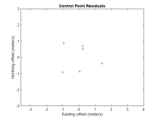
tform = fitgeotform2d(input,spatial,"projective");Compute the 2-D residuals.
residuals = transformPointsForward(tform,input) - spatial;
Plot the 2-D residuals. Add a title and axes labels. Adjust the axes limits.
figure
plot(residuals(:,1),residuals(:,2),"+")

title("Control Point Residuals")
xlabel("Easting offset (meters)")
ylabel("Northing offset (meters)")

xlim([-3 3])
ylim([-3 3])
axis equal
Predict the corner point locations of the registered image in map coordinates.
mInput = size(inputImage,1);
nInput = size(inputImage,2);

inputCorners = 0.5 + [0 0; 0 mInput; nInput mInput; nInput 0; 0 0];

outputCornersSpatial = transformPointsForward(tform,inputCorners);
outputCornersX = outputCornersSpatial(:,1);
outputCornersY = outputCornersSpatial(:,2);
Display the outline of the image on the map by connecting the corner points.
figure(ax1.Parent)
line(outputCornersX,outputCornersY,Color="w")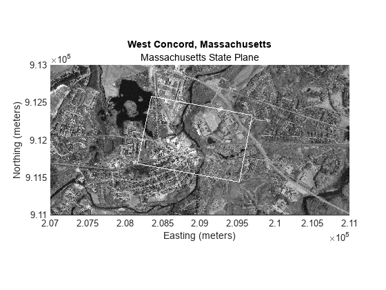
Calculate the average pixel size of the input image in map units.
pixelSize = [hypot( ...
    outputCornersX(2) - outputCornersX(1), ...
    outputCornersY(2) - outputCornersY(1)) / mInput, ...
 hypot( ...
    outputCornersX(4) - outputCornersX(5), ...
    outputCornersY(4) - outputCornersY(5)) / nInput]
pixelSize = 1×2

    0.9020    0.8959
The average pixel size provides a starting point from which to select a width and height for the pixels in the georeferenced output image. In principle, the output pixels can be any size. However, if you make the pixel size too small, you might waste memory and computation time, and create a blurry image. If you make the pixel size too big, then you might alias the image or needlessly discard information from the original image. In general, you also want the pixels to be square. A reasonable heuristic is to select a "reasonable" number (i.e., 0.95 or 1.0 rather than 0.9020) that is slightly larger than the maximum average pixel size.
For this example, specify a pixel size of 1, which means that each pixel in the georeferenced image covers one square meter on the ground. Georeferenced images that align along integer map coordinates are convenient for display and analysis.
outputPixelSize = 1;
Choose world limits that are integer multiples of the output pixel size.
xWorldLimits = outputPixelSize ...
    * [floor(min(outputCornersX) / outputPixelSize), ...
        ceil(max(outputCornersX) / outputPixelSize)]
xWorldLimits = 1×2

      208163      209699
yWorldLimits = outputPixelSize ...
    * [floor(min(outputCornersY) / outputPixelSize), ...
        ceil(max(outputCornersY) / outputPixelSize)]
yWorldLimits = 1×2

      911437      912581
Display the bounding box for the registered image.
line(xWorldLimits([1 1 2 2 1]),yWorldLimits([2 1 1 2 2]),Color="red")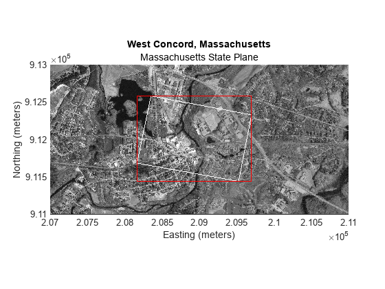
Calculate the dimensions of the registered image.
mOutput = diff(yWorldLimits) / outputPixelSize
mOutput =
1144
nOutput = diff(xWorldLimits) / outputPixelSize
nOutput =
1536
Create an Image Processing Toolbox referencing object for the registered image.
Rimage = imref2d([mOutput nOutput],xWorldLimits,yWorldLimits)
Rimage =
  imref2d with properties:

           XWorldLimits: [208163 209699]
           YWorldLimits: [911437 912581]
              ImageSize: [1144 1536]
    PixelExtentInWorldX: 1
    PixelExtentInWorldY: 1
    ImageExtentInWorldX: 1536
    ImageExtentInWorldY: 1144
       XIntrinsicLimits: [0.5000 1.5365e+03]
       YIntrinsicLimits: [0.5000 1.1445e+03]
Create a map raster reference object for the registered image, which is the Mapping Toolbox counterpart to an Image Processing Toolbox referencing object.
Rmap = maprefcells(Rimage.XWorldLimits,Rimage.YWorldLimits,Rimage.ImageSize, ...
    ColumnsStartFrom="north")
Rmap =
  MapCellsReference with properties:

            XWorldLimits: [208163 209699]
            YWorldLimits: [911437 912581]
              RasterSize: [1144 1536]
    RasterInterpretation: 'cells'
        ColumnsStartFrom: 'north'
           RowsStartFrom: 'west'
      CellExtentInWorldX: 1
      CellExtentInWorldY: 1
    RasterExtentInWorldX: 1536
    RasterExtentInWorldY: 1144
        XIntrinsicLimits: [0.5 1536.5]
        YIntrinsicLimits: [0.5 1144.5]
      TransformationType: 'rectilinear'
    CoordinateSystemType: 'planar'
            ProjectedCRS: []
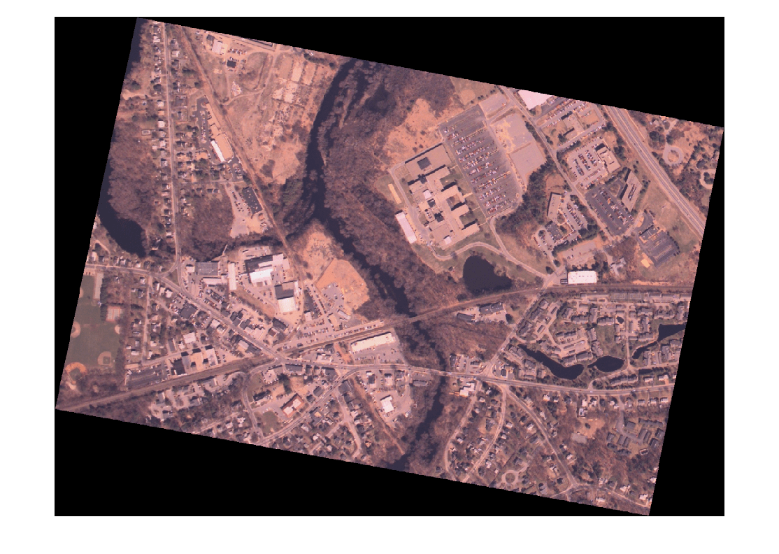
Apply the geometric transformation by using the imwarp function. Flip the output so that the columns run from north to south.
registered = flipud(imwarp(inputImage,tform,OutputView=Rimage));

figure
imshow(registered)
Write the registered image to a TIFF file. Write the spatial referencing information to a world file.
imwrite(registered,"concord_aerial_sw_reg.tif");
worldfilewrite(Rmap,getworldfilename("concord_aerial_sw_reg.tif"));
Display Registered Image in Map Coordinates
Create a new map of the orthophoto base tiles.
figure
mapshow(baseImage,cmap,R)

title("West Concord, Massachusetts")
subtitle("Massachusetts State Plane")

xlabel("Easting (meters)")
ylabel("Northing (meters)")
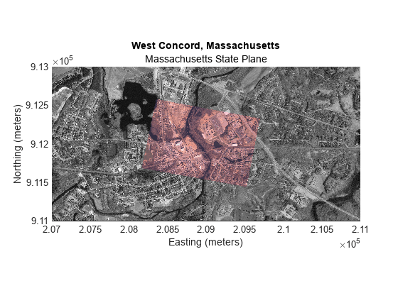
Display the registered image on the same map. The registered image does not completely fill its bounding box, so the image includes missing data. Render the missing data as transparent by creating an alpha data mask. You can assess the registration by looking at features that span both the registered image and the orthophoto images.
alphaData = registered(:,:,1);
alphaData(alphaData~=0) = 255;

ax2 = gca;
mInput = mapshow(ax2,registered,Rmap);
mInput.AlphaData = alphaData;
Overlay Vector Road Layer
Specify the name of a shapefile that contains road data for an area around West Concord. Get information about the shapefile by using the shapeinfo function. Read the data into the workspace as a geospatial table by using the readgeotable function.
roadsfile = "concord_roads.shp";
roadinfo = shapeinfo(roadsfile);
roads = readgeotable(roadsfile);
Create a symbol specification that hides minor roads. Then, display the roads on the same map. Note that the roads in the shapefile generally align with the roads in the images. The two obvious linear features that are not represented by the shapefile data are railroads.
roadspec = makesymbolspec("Line",{'CLASS',6,'Visible','off'});
mapshow(roads,SymbolSpec=roadspec,Color="cyan")

See Also
Functions
readgeoraster|im2uint8(Image Processing Toolbox) |cpstruct2pairs(Image Processing Toolbox) |intrinsicToWorld|fitgeotform2d(Image Processing Toolbox) |transformPointsForward(Image Processing Toolbox) |imref2d(Image Processing Toolbox)