qz

R2026b

Generalized Schur (QZ) factorization for generalized eigenvalues

Syntax

[AA,BB,Q,Z] = qz(A,B)

[AA,BB,Q,Z,V,W] = qz(A,B)

[___] = qz(A,B,mode)

Description

[AA,BB,Q,Z] = qz(A,B) performs a QZ factorization on square matrices A and B such that Q*A*Z = AA and Q*B*Z = BB.

• If A and B are real, then AA and BB are upper quasitriangular matrices.

• If A and B are complex, then AA and BB are triangular.

• Q and Z are unitary matrices.

[AA,BB,Q,Z,V,W] = qz(A,B) also returns matrices V and W whose columns are the right and left generalized eigenvectors, respectively, for A and B.

[___] = qz(A,B,mode) returns a real decomposition if mode is "real" or returns a possibly complex decomposition if mode is "complex". Use this syntax with any of the output argument combinations in the previous syntaxes.

Examples

QZ Factorization

Calculate the QZ factorization of two 3-by-3 matrices.

A = [1 7 3; 2 9 12; 5 22 7];
B = [3 1 0; 0 3 1; 0 0 3];
[AA,BB,Q,Z] = qz(A,B)

AA = 3×3

   23.5574    1.4134  -14.3485
         0   -0.5776    2.7629
         0         0   -8.6720

BB = 3×3

    3.5845   -0.1090   -0.6024
         0    2.7599    0.8430
         0         0    2.7292

Q = 3×3

    0.2566    0.6353    0.7284
   -0.9477    0.3134    0.0604
   -0.1899   -0.7058    0.6824

Z = 3×3

    0.1502   -0.9664   -0.2088
    0.4689    0.2556   -0.8455
    0.8704    0.0291    0.4915

Verify that the norms of AA - Q*A*Z, BB - Q*B*Z, Q'*Q - eye(size(Q)), and Z'*Z - eye(size(Z)) are 0, within machine precision.

norm(AA - Q*A*Z)

ans = 
6.3184e-15

norm(BB - Q*B*Z)

ans = 
1.7936e-15

norm(Q'*Q - eye(size(Q)))

ans = 
8.8320e-16

norm(Z'*Z - eye(size(Z)))

ans = 
5.1071e-16

Generalized Eigenvectors

Calculate the QZ factorization and also return the generalized eigenvectors of two 2-by-2 matrices.

A = [10 -7; -3 2];
B = [7 3; 12 9];
[AA,BB,Q,Z,V,W] = qz(A,B)

AA = 2×2

   11.9600   -4.3532
         0   -0.0836

BB = 2×2

    1.6381   -2.9374
         0   16.4830

Q = 2×2

   -0.9597    0.2811
    0.2811    0.9597

Z = 2×2

   -0.5752    0.8180
    0.8180    0.5752

V = 2×2

   -0.7031    0.6960
    1.0000    1.0000

W = 2×2

   -1.0000    0.2929
    0.4537    1.0000

Verify that the elements of Q*A*Z - AA and Q*B*Z - BB are 0, within machine precision.

Q*A*Z - AA

ans = 2×2
10-14 ×

         0    0.1776
   -0.1034   -0.1180

Q*B*Z - BB

ans = 2×2
10-14 ×

   -0.0222         0
    0.0888   -0.3553

Calculate the generalized eigenvalues and right and left eigenvectors of A and B by using the eig function. Verify that the elements of A*V - B*V*D and W'*A - D*W'*B are 0, within machine precision.

[V,D,W] = eig(A,B);
A*V - B*V*D

ans = 2×2
10-14 ×

         0   -0.2054
   -0.7105   -0.0333

W'*A - D*W'*B

ans = 2×2
10-14 ×

    0.7105   -0.3553
   -0.0805   -0.0319

Complex QZ Factorization

Calculate the complex QZ factorization of two 3-by-3 matrices.

A = [1/sqrt(2) 1 0; 0 1 1; 0 1/sqrt(2) 1];
B = [0 1 1; -1/sqrt(2) 0 1; 1 -1/sqrt(2) 0];
[AAc,BBc,Qc,Zc] = qz(A,B)

AAc = 3×3 complex

   0.5011 - 0.8679i   0.0332 - 1.0852i   0.3687 + 0.9278i
   0.0000 + 0.0000i   0.1848 - 0.0000i  -0.6334 - 0.3673i
   0.0000 + 0.0000i   0.0000 + 0.0000i   0.5590 + 0.9682i

BBc = 3×3 complex

   1.0022 + 0.0000i   0.3136 + 0.0711i  -0.0280 + 0.5966i
   0.0000 + 0.0000i   1.3388 + 0.0000i   0.1572 + 0.6846i
   0.0000 + 0.0000i   0.0000 + 0.0000i   1.1180 + 0.0000i

Qc = 3×3 complex

   0.5379 + 0.2210i   0.4604 - 0.3553i   0.3214 - 0.4693i
   0.2172 + 0.3386i   0.4018 - 0.0188i  -0.7698 + 0.2895i
  -0.3719 - 0.6014i   0.7068 - 0.0213i  -0.0000 - 0.0000i

Zc = 3×3 complex

   0.2514 + 0.0413i  -0.7279 - 0.4531i  -0.4470 - 0.0135i
  -0.1000 - 0.6068i   0.3328 - 0.3332i  -0.3326 + 0.5379i
   0.6391 + 0.3853i   0.1423 - 0.1511i   0.2996 + 0.5570i

Calculate the real QZ decomposition of A and B by specifying mode as "real". The generalized Schur form of A is quasitriangular, indicating that it has complex eigenvalues.

[AAr,BBr,Qr,Zr] = qz(A,B,"real")

AAr = 3×3

    0.1464    1.1759    0.3094
         0    1.0360    1.2594
         0   -0.8587    0.3212

BBr = 3×3

    1.0607   -0.5952    0.1441
         0    1.6676         0
         0         0    0.8481

Qr = 3×3

    0.0000   -0.0000   -1.0000
   -0.7882   -0.6154   -0.0000
   -0.6154    0.7882   -0.0000

Zr = 3×3

   -0.7071    0.2610   -0.6572
    0.5000   -0.4727   -0.7257
   -0.5000   -0.8417    0.2037

For triangular AAc, compute the eigenvalues by using diag(AA)./diag(BB).

diag(AAc)./diag(BBc)

ans = 3×1 complex

   0.5000 - 0.8660i
   0.1381 - 0.0000i
   0.5000 + 0.8660i

For quasitriangular AAr, compute the eigenvalues by using the ordeig function.

ordeig(AAr,BBr)

ans = 3×1 complex

   0.1381 + 0.0000i
   0.5000 + 0.8660i
   0.5000 - 0.8660i

Input Arguments

A, B — Input matrices

square matrices

Input matrices, specified as real or complex square matrices. The dimensions of A and B must be the same.

Data Types: single | double
Complex Number Support: Yes

mode — Decomposition mode

"complex" (default) | "real"

Decomposition mode, specified as one of these values:

• "complex" — qz returns a possibly complex decomposition, and AA and BB are triangular.

• "real" — qz returns a real decomposition, and AA and BB are quasitriangular.

Output Arguments

AA, BB — Generalized Schur forms of A and B

square matrices

Generalized Schur forms of A and B, returned as upper triangular or quasitriangular square matrices.

• When the decomposition is complex and AA is triangular, then the diagonal elements a = diag(AA) and b = diag(BB) are the generalized eigenvalues that satisfy A*V*b = B*V*a and b'*W'*A = a'*W'*B.

• When the decomposition is real and AA is quasitriangular, you must further reduce the 2-by-2 blocks to obtain the eigenvalues of the full system. Each 2-by-2 block in AA corresponds to a 2-by-2 diagonal block at the same location in BB.

Q, Z — Unitary factors

square matrices

Unitary factors, returned as square matrices that satisfy Q*A*Z = AA and Q*B*Z = BB.

V — Right eigenvectors

square matrix

Right eigenvectors, returned as a square matrix whose columns are the generalized right eigenvectors of the pair (A,B).

• When mode is "complex" (the default mode), the eigenvectors satisfy A*V = B*V*D, where D contains the generalized eigenvalues of the pair along its main diagonal.

• When mode is "real", the eigenvectors might need to be reconstructed to satisfy A*V = B*V*D. For more information, see Eigenvector Reconstruction.

Use the eig function to return D and the ordeig function to return the diagonal elements of D. Eigenvalues and eigenvectors returned by qz and eig might be ordered or normalized differently.

Different machines and releases of MATLAB^® can produce different eigenvectors that are still numerically accurate:

• For real eigenvectors, the sign of the eigenvectors can change.

• For complex eigenvectors, the eigenvectors can be multiplied by any complex number of magnitude 1.

• For a multiple eigenvalue, its eigenvectors can be recombined through linear combinations. For example, if Ax = λx and Ay = λy, then A(x+y) = λ(x+y), so x+y also is an eigenvector of A.

W — Left eigenvectors

square matrix

Left eigenvectors, returned as a square matrix whose columns are the generalized left eigenvectors of the pair (A,B).

• When mode is "complex" (the default mode), the eigenvectors satisfy W'*A = D*W'*B, where D contains the generalized eigenvalues of the pair along its main diagonal.

• When mode is "real", the eigenvectors might need to be reconstructed to satisfy W'*A = D*W'*B. For more information, see Eigenvector Reconstruction.

Use the eig function to return D and the ordeig function to return the diagonal elements of D. Eigenvalues and eigenvectors returned by qz and eig might be ordered or normalized differently.

Different machines and releases of MATLAB can produce different eigenvectors that are still numerically accurate:

• For real eigenvectors, the sign of the eigenvectors can change.

• For complex eigenvectors, the eigenvectors can be multiplied by any complex number of magnitude 1.

• For a multiple eigenvalue, its eigenvectors can be recombined through linear combinations. For example, if Ax = λx and Ay = λy, then A(x+y) = λ(x+y), so x+y also is an eigenvector of A.

More About

Quasitriangular Matrix

An upper quasitriangular matrix can result from the Schur decomposition or generalized Schur (QZ) decomposition of a real matrix. An upper quasitriangular matrix is block upper triangular, with 1-by-1 and 2-by-2 blocks of nonzero values along the diagonal.

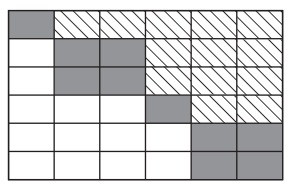
The eigenvalues of these diagonal blocks are also the eigenvalues of the matrix. The 1-by-1 blocks correspond to real eigenvalues, and the 2-by-2 blocks correspond to complex conjugate eigenvalue pairs.

Unitary Matrix

An invertible complex square matrix U is unitary if its conjugate transpose is also its inverse, that is, if $$U^{*}U=U{U}^{*}=I$$.

Eigenvector Reconstruction

When mode is "real" and the input matrices A and B have at least one complex conjugate pair of eigenvalues, the returned eigenvectors V and W generally do not satisfy A*V = B*V*D and W'*A = D*W'*B.

To reconstruct the eigenvectors so that they satisfy these equations, combine adjacent columns of V and W into pairs conjugate eigenvectors. If you reconstruct the eigenvectors, the equations are satisfied for D = diag(ordeig(AA,BB)).

For example, this code reconstructs the left and right eigenvector matrix output from the function call [AA,BB,Q,Z,V,W] = qz(A,B,"real"). These reconstructed eigenvector matrices are equivalent to those returned by [V,D,W] = eig(A,B), although the order of eigenvalues and normalization of eigenvectors might be different.

for i=1:n-1
    if AA(i+1,i) == 0
        continue;
    end
    V(:,i:i+1) = V(:,i:i+1) * [1 1; 1i -1i];
    W(:,i:i+1) = W(:,i:i+1) * [1 1; 1i -1i];
end

Tips

• You can calculate the generalized eigenvalues that solve the generalized eigenvalue problem $$Ax=\lambda Bx$$ from the QZ factorization. For triangular AA, calculate the eigenvalues using diag(AA)./diag(BB). For quasitriangular AA, calculate the eigenvalues using ordeig(AA,BB).

Extended Capabilities

Thread-Based Environment

Run code in the background using MATLAB® backgroundPool or accelerate code with Parallel Computing Toolbox™ ThreadPool.

The qz function fully supports thread-based environments. For more information, see Run MATLAB Functions in Thread-Based Environment.

Version History

Introduced before R2006a