Benchmark A\b on the GPU
This example shows how to benchmark the solving of a linear system on the GPU.
Linear algebra functions in MATLAB® provide fast, numerically robust matrix calculations, and the code to solve for x in A*x = b is very simple. You use matrix left division, also known as mldivide or the backslash operator (\), to calculate x (that is, x = A\b). This example compares the single- and double-precision performance of the mldivide function on the GPU and CPU for different matrix sizes.
Check GPU Setup
Check whether a GPU is available.
gpu = gpuDevice;
disp(gpu.Name + " GPU detected and available.")
NVIDIA RTX A5000 GPU detected and available.
The code in this example was timed on a Windows® 11, Intel® Xeon® W-2133 @ 3.60 GHz test system with 64 GB of RAM.
Define Benchmark Parameters
As with a number of other parallel algorithms, the performance of solving a linear system in parallel depends greatly on the matrix size and so it is important to choose appropriate matrix sizes for the benchmark. To define the test parameters:
Create a variable representing the number of bytes required to store a double-precision number.
Specify the maximum number of tests to run.
Create a vector of sizes, where the maximum size is 1/5 of the available GPU memory. The benchmark loops over this vector and creates arrays of increasing size. To create a vector of logarithmically spaced points, use the
logspacefunction.As an array on the GPU in MATLAB cannot have more than elements, remove any sizes that will create arrays larger than this.
sizeOfDouble = 8;
maxNumTests = 15;
maxSize = 0.2*gpu.AvailableMemory;
sizes = logspace(5,log10(maxSize),maxNumTests);
sizes(sizes/sizeOfDouble > intmax) = [];
Run Benchmarks
The number of floating-point operations that a processor can perform per second is a useful measure of performance. To determine the number of floating-point operations per second (FLOPS), divide the number of floating-point operations performed by the time taken to perform those operations.
Use the floating-point operations count of the HPC Challenge, so that for an n-by-n matrix, the number of floating-point operations is
.
Double Precision
MATLAB can perform calculations in double precision or single precision. Calculating in single precision instead of double precision can improve the performance of code running on your GPU, as most GPU cards are designed for graphics display, which demands a high single-precision performance. In contrast, CPUs are designed for general purpose computing and so do not provide as much improvement when switching from double to single precision. For more information on converting data to single precision and performing arithmetic operations on single-precision data, see Floating-Point Numbers. Typical examples of workflows suitable for single-precision computation on the GPU include image processing and machine learning. However, other types of calculation, such as linear algebra problems, typically require double-precision processing.
For an approximate measure of the relative performance of your GPU in single precision compared to double precision, query the SingleDoubleRatio property of your device. This property describes the ratio of single- to double-precision floating-point units (FPUs) on the device. Most desktop GPUs have 24, 32, or even 64 times as many single-precision floating-point units as double-precision.
gpu.SingleDoubleRatio
ans =
32
To benchmark the performance of the GPU and host CPU in double precision, for each array size in sizes:
Create a random double-precision matrix
Aand vectorbon the GPU and on the host. By default, therandandeyefunctions create double-precision arrays.Use the
timeitfunction to timemldivideon the host CPU.Use the
gpuArrayfunction to transferAandbto GPU memory.Use the
gputimeitfunction on the GPU.
numTests = numel(sizes);
NDouble = floor(sqrt(sizes/(sizeOfDouble)));
timeCPUDouble = inf(1,numTests);
timeGPUDouble = inf(1,numTests);

for idx=1:numTests
    disp("Test " + idx + " of " + numTests + ". Timing double-precision mldivide on GPU and CPU with " + NDouble(idx)^2 + " elements.")
    A = rand(NDouble(idx)) + 100*eye(NDouble(idx));
    b = rand(NDouble(idx),1);

    timeCPUDouble(idx) = timeit(@() A\b);

    A = gpuArray(A);
    b = gpuArray(b);
    timeGPUDouble(idx) = gputimeit(@() A\b);
end
Test 1 of 15. Timing double-precision mldivide on GPU and CPU with 12321 elements.
Test 2 of 15. Timing double-precision mldivide on GPU and CPU with 26896 elements.
Test 3 of 15. Timing double-precision mldivide on GPU and CPU with 58564 elements.
Test 4 of 15. Timing double-precision mldivide on GPU and CPU with 126736 elements.
Test 5 of 15. Timing double-precision mldivide on GPU and CPU with 275625 elements.
Test 6 of 15. Timing double-precision mldivide on GPU and CPU with 597529 elements.
Test 7 of 15. Timing double-precision mldivide on GPU and CPU with 1295044 elements.
Test 8 of 15. Timing double-precision mldivide on GPU and CPU with 2808976 elements.
Test 9 of 15. Timing double-precision mldivide on GPU and CPU with 6091024 elements.
Test 10 of 15. Timing double-precision mldivide on GPU and CPU with 13205956 elements.
Test 11 of 15. Timing double-precision mldivide on GPU and CPU with 28633201 elements.
Test 12 of 15. Timing double-precision mldivide on GPU and CPU with 62062884 elements.
Test 13 of 15. Timing double-precision mldivide on GPU and CPU with 134536801 elements.
Test 14 of 15. Timing double-precision mldivide on GPU and CPU with 291623929 elements.
Test 15 of 15. Timing double-precision mldivide on GPU and CPU with 632170449 elements.
Determine the GPU and CPU double-precision processing power in FLOPS.
flopsCPUDouble = (2/3*NDouble.^3 + 3/2*NDouble.^2)./timeCPUDouble;
flopsGPUDouble = (2/3*NDouble.^3 + 3/2*NDouble.^2)./timeGPUDouble;
Single Precision
You can convert data to single precision by using the single function, or by specifying single as the data type in a creation function such as zeros, ones, rand, and eye.
Benchmark the performance of the GPU and host CPU in single precision.
NSingle = floor(sqrt(sizes/(sizeOfDouble/2)));
timeCPUSingle = inf(1,numTests);
timeGPUSingle = inf(1,numTests);

for idx=1:numTests
    disp("Test " + idx + " of " + numTests + ". Timing single-precision mldivide on GPU and CPU with " + NSingle(idx)^2 + " elements.")
    A = rand(NSingle(idx),"single") + 100*eye(NSingle(idx),"single");
    b = rand(NSingle(idx),1,"single");

    timeCPUSingle(idx) = timeit(@() A\b);

    A = gpuArray(A);
    b = gpuArray(b);
    timeGPUSingle(idx) = gputimeit(@() A\b);
end
Test 1 of 15. Timing single-precision mldivide on GPU and CPU with 24964 elements.
Test 2 of 15. Timing single-precision mldivide on GPU and CPU with 53824 elements.
Test 3 of 15. Timing single-precision mldivide on GPU and CPU with 116964 elements.
Test 4 of 15. Timing single-precision mldivide on GPU and CPU with 254016 elements.
Test 5 of 15. Timing single-precision mldivide on GPU and CPU with 550564 elements.
Test 6 of 15. Timing single-precision mldivide on GPU and CPU with 1194649 elements.
Test 7 of 15. Timing single-precision mldivide on GPU and CPU with 2592100 elements.
Test 8 of 15. Timing single-precision mldivide on GPU and CPU with 5621641 elements.
Test 9 of 15. Timing single-precision mldivide on GPU and CPU with 12187081 elements.
Test 10 of 15. Timing single-precision mldivide on GPU and CPU with 26409321 elements.
Test 11 of 15. Timing single-precision mldivide on GPU and CPU with 57259489 elements.
Test 12 of 15. Timing single-precision mldivide on GPU and CPU with 124121881 elements.
Test 13 of 15. Timing single-precision mldivide on GPU and CPU with 269091216 elements.
Test 14 of 15. Timing single-precision mldivide on GPU and CPU with 583270801 elements.
Test 15 of 15. Timing single-precision mldivide on GPU and CPU with 1264371364 elements.
Determine the GPU and CPU single-precision processing power in FLOPS.
flopsCPUSingle = (2/3*NSingle.^3 + 3/2*NSingle.^2)./timeCPUSingle;
flopsGPUSingle = (2/3*NSingle.^3 + 3/2*NSingle.^2)./timeGPUSingle;
Plot the Performance
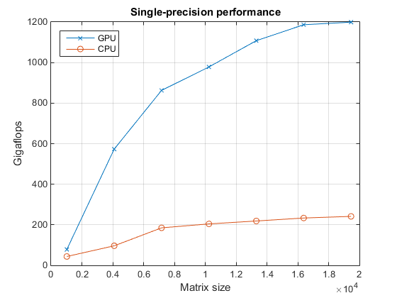
Plot the processing power against array size for double precision and single precision. The performance of both the CPU and GPU plateau at large matrix sizes.
figure
loglog(NDouble.^2,flopsGPUDouble, ...
     NDouble.^2,flopsCPUDouble)
grid on
legend(["GPU" "CPU"],Location="NorthWest")
title("Double-Precision Performance","\fontname{monospace}mldivide")
ylabel("Calculation Rate (FLOPS)")
xlabel("Matrix Size (number of elements)")

figure
loglog(NSingle.^2,flopsGPUSingle, ...
     NSingle.^2,flopsCPUSingle)
grid on
legend(["GPU" "CPU"],Location="NorthWest")
title("Single-Precision Performance","\fontname{monospace}mldivide")
ylabel("Calculation Rate (FLOPS)")
xlabel("Matrix Size (number of elements)")

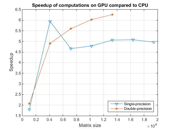
Calculate the ratio of CPU execution time to GPU execution time (the speedup) and plot the results. Plot a line indicating a speedup of one. Points above this line indicate matrix sizes for which mldivide is faster on the GPU than on the CPU. As the GPU used to publish this example has less memory than the CPU, the performance on the GPU becomes limited by memory latency at smaller matrix sizes than on the CPU. Memory latency is the time it takes to transfer data from memory to the floating-point units.
speedupDouble = timeCPUDouble./timeGPUDouble;
speedupSingle = timeCPUSingle./timeGPUSingle;

figure
semilogx(NSingle.^2,speedupSingle, ...
     NDouble.^2,speedupDouble)
yline(1,"--")

grid on
legend(["Single precision" "Double precision"],Location="NorthWest")
title("Speedup of Computations on GPU Compared to CPU")
ylabel("Speedup")
xlabel("Matrix Size (number of elements)")

These benchmarks show that:
Given large enough data, a GPU can perform calculations faster than the host CPU.
GPUs perform calculations faster in single precision than double precision, and often much faster.
The results of these benchmarks will vary based on your hardware.
See Also
gpuArray | gpuDevice | mldivide