Heat Distribution in Circular Cylindrical Rod: PDE Modeler App

Solve a 3-D parabolic PDE problem by reducing the problem to 2-D using coordinate transformation. This example uses the PDE Modeler app. For the command-line solution, see Heat Distribution in Circular Cylindrical Rod.

Consider a cylindrical radioactive rod. Heat is continuously added at the left end of the rod, while the right end is kept at a constant temperature. At the outer boundary, heat is exchanged with the surroundings by transfer. At the same time, heat is uniformly produced in the whole rod due to radioactive processes. Assuming that the initial temperature is zero leads to the following equation:

$ρ C \frac{\partial u}{\partial t} - \nabla \cdot (k \nabla u) = q$

Here, ρ, C, and k are the density, thermal capacity, and thermal conductivity of the material, u is the temperature, and q is the heat generated in the rod.

Since the problem is axisymmetric, it is convenient to write this equation in a cylindrical coordinate system.

$ρ C \frac{\partial u}{\partial t} - \frac{1}{r} \frac{\partial}{\partial r} (k r \frac{\partial u}{\partial r}) - \frac{1}{r^{2}} \frac{\partial}{\partial θ} (k \frac{\partial u}{\partial θ}) - \frac{\partial}{\partial z} (k \frac{\partial u}{\partial z}) = q$

Here r, θ, and z are the three coordinate variables of the cylindrical system. Because the problem is axisymmetric, $\partial u / \partial θ = 0$ .

This is a cylindrical problem, and Partial Differential Equation Toolbox™ requires equations to be in Cartesian coordinates. To transform the equation to the Cartesian coordinates, first multiply both sides of the equation by r:

$ρ r C \frac{\partial u}{\partial t} - \frac{\partial}{\partial r} (k r \frac{\partial u}{\partial r}) - \frac{\partial}{\partial z} (k r \frac{\partial u}{\partial z}) = q r$

Then define r as y and z as x:

$ρ y C \frac{\partial u}{\partial t} - \nabla \cdot (k y \nabla u) = q y$

For this example, use these parameters:

Density, ρ = 7800 kg/m³
Thermal capacity, C = 500 W·s/kg·ºC
Thermal conductivity, k = 40 W/mºC
Radioactive heat source, q = 20000 W/m³
Temperature at the right end, T_right = 100 ºC
Heat flux at the left end, HF_left = 5000 W/m²
Surrounding temperature at the outer boundary, T_outer = 100 ºC
Heat transfer coefficient, h_outer = 50 W/m²·ºC

To solve this problem in the PDE Modeler app, follow these steps:

Model the rod as a rectangle with corners in (-1.5,0), (1.5,0), (1.5,0.2), and (-1.5,0.2). Here, the x-axis represents the z direction, and the y-axis represents the r direction.
```
pderect([-1.5,1.5,0,0.2])
```
Specify the boundary conditions. To do this, double-click the boundaries to open the Boundary Condition dialog box. The PDE Modeler app requires boundary conditions in a particular form. Thus, Neumann boundary conditions must be in the form $\vec{n} \cdot (c \nabla u) + q u = g$ , and Dirichlet boundary conditions must be in the form hu = r. Also, because both sides of the equation are multiplied by r = y, multiply coefficients for the boundary conditions by y.
- For the left end, use the Neumann condition $\vec{n} \cdot (k \nabla u) = H F_l e f t = 5000$ . Specify g = 5000*y and q = 0.
- For the right end, use the Dirichlet condition u = T_right = 100. Specify h = 1 and r = 100.
- For the outer boundary, use the Neumann condition $\vec{n} \cdot (k \nabla u) = h_o u t e r (T_o u t e r - u) = 50 (100 - u)$ . Specify g = 50*y*100 and q = 50*y.
- The cylinder axis r = 0 is not a boundary in the original problem, but in the 2-D treatment it has become one. Use the artificial Neumann boundary condition for the axis, $\vec{n} \cdot (k \nabla u) = 0$ . Specify g = 0 and q = 0.
Specify the coefficients by selecting PDE > PDE Specification or click the button on the toolbar. Heat equation is a parabolic equation, so select the Parabolic type of PDE. Because both sides of the equation are multiplied by r = y, multiply the coefficients by y and enter the following values: c = 40*y, a = 0, f = 20000*y, and d = 7800*500*y.
Initialize the mesh by selecting Mesh > Initialize Mesh.
Refine the mesh by selecting Mesh > Refine Mesh.
Set the initial value to 0, the solution time to 20000 seconds, and compute the solution every 100 seconds. To do this, select Solve > Parameters. In the Solve Parameters dialog box, set time to 0:100:20000, and u(t₀) to 0.
Solve the equation by selecting Solve > Solve PDE or clicking the button on the toolbar.
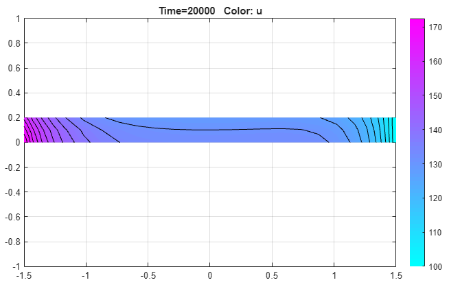
Plot the solution, using the color and contour plot. To do this, select Plot > Parameters and choose the color and contour plots in the resulting dialog box.

You can explore the solution by varying the parameters of the model and plotting the results. For example, you can:

Show the solution when u does not depend on time, that is, the steady state solution. To do this, open the PDE Specification dialog box, and change the PDE type to Elliptic. The resulting steady state solution is in close agreement with the transient solution at 20000 seconds.
Show the steady state solution without cooling on the outer boundary: the heat transfer coefficient is zero. To do this, set the Neumann boundary condition at the outer boundary (the top side of the rectangle) to g = 0 and q = 0. The resulting plot shows that the temperature rises to more than 2500 on the left end of the rod.