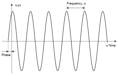
Rectangular, Triangular, Trapezoidal, and Harmonic Loads

Model rectangular, triangular, trapezoidal, and harmonic loads by creating the helper functions. By using different parameters, such as start, rise, fall, and end times and also frequency and phase, you can model a variety of loads.

Rectangular, Triangular, and Trapezoidal Pulses

Model a trapezoidal pulse load by specifying its magnitude and a set of times.

Define a trapezoidal pulse function, trapezoidalLoad, to model a trapezoidal load. This function accepts the load magnitude, the location and state structure arrays, and the function specifying the pulse parameters that define the start, rise, fall, and end times. Because the function depends on time, it must return a matrix of NaN of the correct size when state.time is NaN. Solvers check whether a problem is nonlinear or time-dependent by passing NaN state values and looking for returned NaN values.

function Tn = trapezoidalLoad(load,location,state,T)
if isnan(state.time)
    Tn = NaN*(location.nx);
    return
end
if isa(load,"function_handle")
    load = load(location,state);
else
    load = load(:);
end
% Four time-points that define a trapezoidal pulse
T1 = T(1); % Start time
T2 = T(2); % Rise time
T3 = T(3); % Fall time
T4 = T(4); % End time

% Determine multiplicative factor for the specified time
TnTrap = max([
    min([(state.time - T1)/(T2-T1), ...
    1, ...
    (T4 - state.time)/(T4-T3)]), ...
    0]);
Tn = load.* TnTrap;
end

The setUpTrapezoid helper function accepts the name-value arguments StartTime, RiseTime, FallTime, and EndTime and processes these parameters for use in the trapezoidalLoad function. Pass the output of this function as the last argument of trapezoidalLoad. The default StartTime, RiseTime, and FallTime values are 0, while the default EndTime value is Inf.

function T = setUpTrapezoid(opts)
arguments
    opts.StartTime double {mustBeScalarOrEmpty,mustBeReal} = []
    opts.RiseTime  double {mustBeScalarOrEmpty,mustBeReal} = []
    opts.FallTime  double {mustBeScalarOrEmpty,mustBeReal} = []
    opts.EndTime   double {mustBeScalarOrEmpty,mustBeReal} = []
end
if isempty(opts.StartTime)
    opts.StartTime = 0;
end
if isempty(opts.RiseTime)
    opts.RiseTime = 0;
end
if isempty(opts.FallTime)
    opts.FallTime = 0;
end
if isempty(opts.EndTime) && (opts.FallTime ~= 0)
    opts.EndTime = opts.StartTime + opts.RiseTime + opts.FallTime;
elseif isempty(opts.EndTime) && (opts.FallTime == 0)
    opts.EndTime = Inf;
end
T = [opts.StartTime;
     opts.StartTime + opts.RiseTime;
     opts.EndTime - opts.FallTime;
     opts.EndTime];
end

As an example, apply a trapezoidal pressure load on face 1 by using these functions.

load = 5e6;
T = setUpTrapezoid(StartTime=1, ...
                   RiseTime=0.5, ...
                   FallTime=0.5, ...
                   EndTime=3);
pressurePulse = @(location,state) ...
                  trapezoidalLoad(load,location,state,T);
model.FaceLoad(1) = faceLoad(Pressure=pressurePulse);

For rectangular and triangular pulses, use the same helper functions and specify start, rise, fall, and end times as follows:

• For a rectangular pulse, specify the start and end times.

• For a triangular pulse, specify the start time and any two of these times: rise time, fall time, and end time. You also can specify all four times, but they must be consistent.

Harmonic Load

Model a harmonic load by specifying its magnitude, frequency, and phase.

Define a sinusoidal load function, sinusoidalLoad, to model a harmonic load. This function accepts the load magnitude (amplitude), the location and state structure arrays, frequency, and phase. Because the function depends on time, it must return a matrix of NaN of the correct size when state.time is NaN. Solvers check whether a problem is nonlinear or time-dependent by passing NaN state values and looking for returned NaN values.

function Tn = sinusoidalLoad(load,location,state,Frequency,Phase)
if isnan(state.time)
    Tn = NaN*(location.nx);
    return
end
if isa(load,"function_handle")
    load = load(location,state);
else
    load = load(:);
end
% Transient model excited with harmonic load
Tn = load.*sin(Frequency.*state.time + Phase);
end

As an example, apply a sinusoidal pressure load on face 1 by using the sinusoidalLoad function.

Pressure = 5e7;
Frequency = 25;
Phase = 0;
pressurePulse = @(location,state) ...
         sinusoidalLoad(Pressure,location,state,Frequency,Phase);
model.FaceLoad(1) = faceLoad(Pressure=pressurePulse);

You can also define a sinusoidal load function depending on all three coordinates.

function Tn = sinusoidalLoad(load,location,state,Frequency,Phase)
if isnan(state.time)
    normal = [location.nx location.ny];
    if isfield(location,"nz")
        normal = [normal location.nz];
    end
    Tn = NaN*normal;
    return
end
if isa(load,"function_handle")
    load = load(location,state);
else
    load = load(:);
end
% Transient model excited with harmonic load
Tn = load.*sin(Frequency.*state.time + Phase);
end

Related Topics

• Nonconstant Parameters of Finite Element Model