Solve Heat Equation Using Graph Neural Network
This example shows how to train a graph neural network (GNN) that solves the heat equation.
A graph neural network (GNN) is a neural network that takes graph structures as input. Graph data is typically represented as a set of node coordinates and a corresponding adjacency matrix. An adjacency matrix is a useful representation that helps to perform accumulation operations across connected nodes, such as graph convolution operations.
The heat equation is a partial differential equation (PDE). The equation models how the temperature evolves in time according to material properties such as the thermal conductivity , specific heat , mass density , and internal heat sources . This example trains a neural network that models the temperature of a material at time for the spatial coordinates in a two-dimensional block with a cavity. The temperature evolves according to the heat equation
.
Using a GNN to predict the solutions of a PDE can be faster than computing the PDE solutions numerically. However, the GNN requires a data set of training data and time to train, and the predicted solutions can be less accurate than solutions computed numerically.
In general, the heat equation holds for , where is a geometric domain, such as the interior of a component. The temperature also depends on initial conditions (the values of for ) and boundary conditions (the values of for ). Boundary conditions are often specified as Dirichlet boundary conditions for the temperature on the boundary ( for ), or as Neumann boundary conditions on the heat flux (, where is the directional derivative in the direction of the outward-pointing normal to the boundary at ).
This example considers a rectangular domain with a smaller rectangular cavity for the case when , , , and . In this case, the heat equation is
,
where is the Laplace operator.
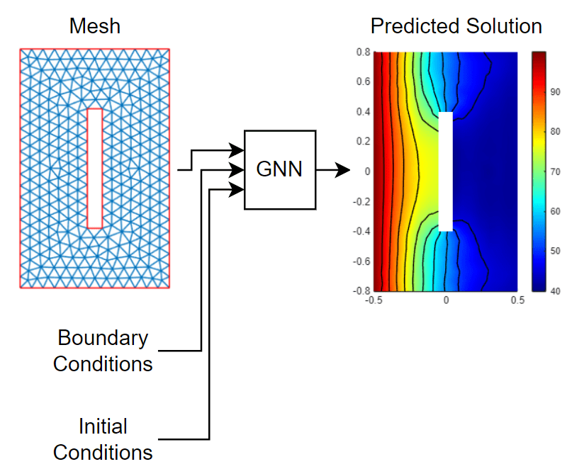
Using a data set of constant initial conditions, boundary conditions, and corresponding solutions, the example trains a GNN that approximates the mapping , where is the initial temperature, is the left-edge temperature, and is the right-edge heat flux. This example generates the training data by defining a PDE using Partial Differential Equation Toolbox™ and solving the PDE for a set of initial and boundary conditions.
To train the GNN, the example groups together the coordinate samples into a graph , where the edges of the graph are defined by a finite element mesh.
This diagram illustrates data flowing through the neural network.
Generate Training Data
Load the initial and boundary conditions. Read the data from the file HeatEquationConditions.csv, which contains values for the initial temperature , left-edge temperature and right-edge heat flux .
initialAndBoundaryConditions = ...
    readtable("HeatEquationConditions.csv", ...
               VariableNamingRule="preserve");
View the first few rows of the data.
head(initialAndBoundaryConditions)
    Initial Condition    E6_Temperature    E1_HeatFlux
    _________________    ______________    ___________

            0                  50              -20
            0                 100              -20
            0                 150              -20
            0                 200              -20
            0                 250              -20
            0                 300              -20
            0                 350              -20
            0                 400              -20
To define the mesh domain for the heat equation, create a PDE model, specify the geometry, and extract the mesh graph. Create the model using the femodel function. To model the evolution of the temperature over time, use a thermal transient model. Specify the model geometry using the crackg function.
thermalmodel = femodel( ...
    AnalysisType="thermalTransient", ...
    Geometry=@crackg);
Specify the material properties of the model. Specify the thermal conductivity , mass density , and specific heat as 1.
thermalmodel.MaterialProperties = materialProperties( ...
    ThermalConductivity=1, ...
    MassDensity=1, ...
    SpecificHeat=1);
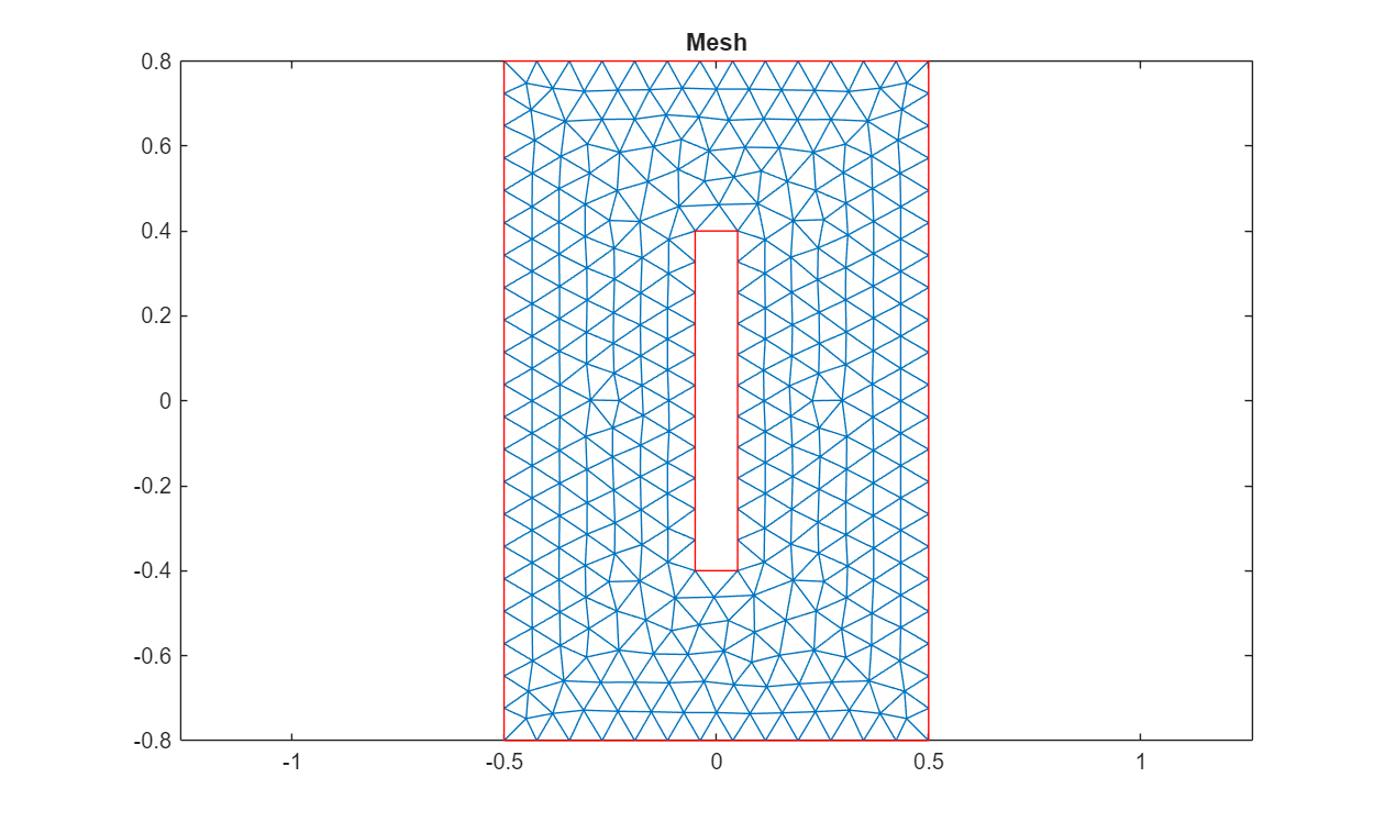
Generate the mesh with a linear geometric order and visualize it in a plot.
thermalmodel = generateMesh(thermalmodel,GeometricOrder="linear");
pdemesh(thermalmodel)
title("Mesh")
Solve the PDE for various initial and boundary conditions.
Specify times to output the solution of the PDE.
solutionTimes = [0 0.1];
Extract the initial conditions, Dirichlet boundary, and Neumann boundary from the training data.
initialCondition = initialAndBoundaryConditions.("Initial Condition");
dirichletBoundary = initialAndBoundaryConditions.E6_Temperature;
neumannBoundary = initialAndBoundaryConditions.E1_HeatFlux;
Solve the PDE by looping over the observations. For each observation, set the initial condition, left-edge boundary condition, and right-edge boundary condition. Then solve the PDE using the solve function and specify the solution times.
numObservations = height(initialAndBoundaryConditions);
solution = cell(1,numObservations);

for i = 1:numObservations
    thermalmodel.FaceIC = faceIC(Temperature=initialCondition(i));

    thermalmodel.EdgeBC(6) = edgeBC(Temperature=dirichletBoundary(i));

    thermalmodel.EdgeLoad(1) = edgeLoad(Heat=neumannBoundary(i));

    solution{i} = solve(thermalmodel,solutionTimes);
end
Visualize one of the observations in a plot. Plot a heat map of one of the solutions at time .
figure
pdeplot(solution{1}.Mesh, ...
    XYData=solution{1}.Temperature(:,end), ...
    Contour="on", ...
    ColorMap="jet");
title("PDE Solution")
axis equal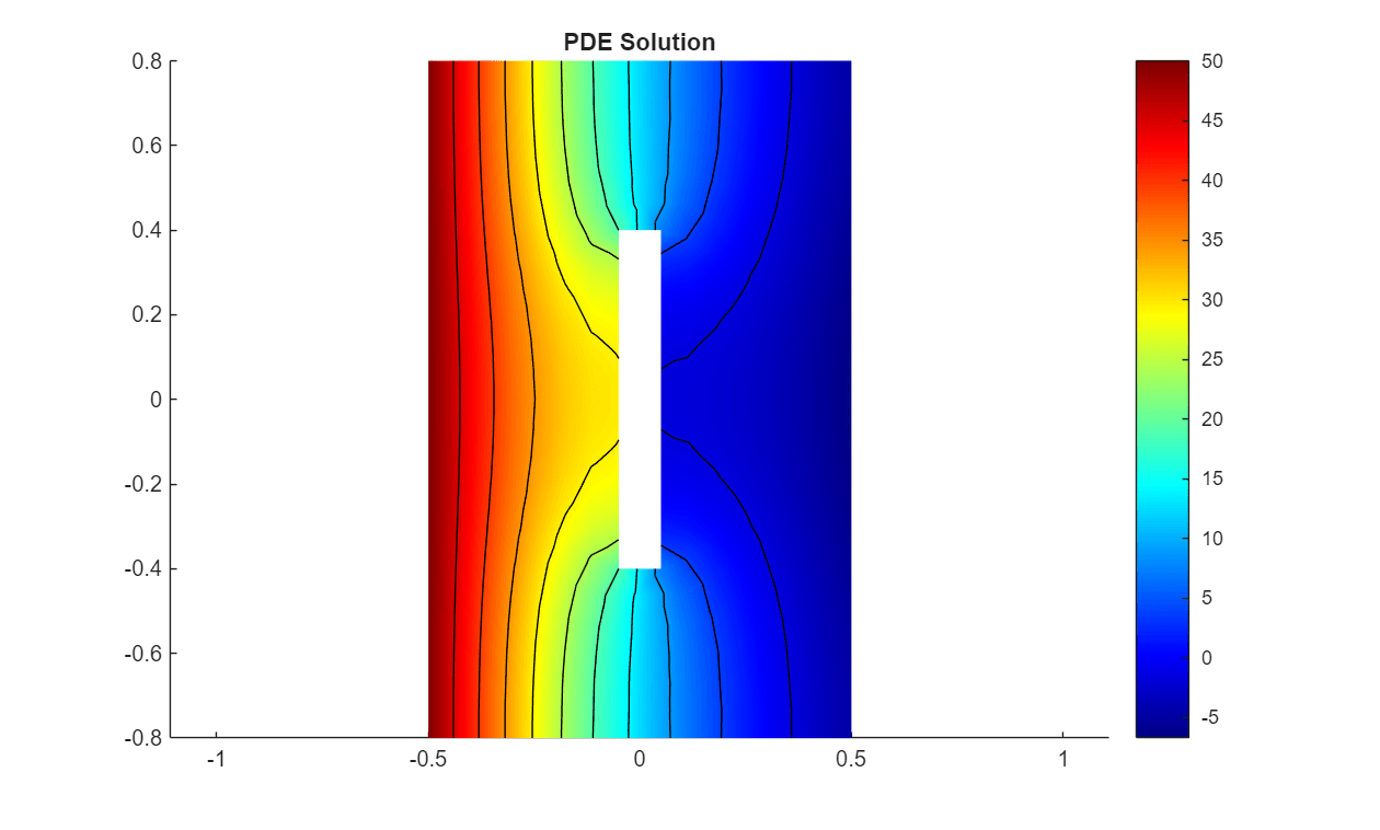
Create an undirected graph using the mesh and find its adjacency matrix. To prevent subsequent gradients from vanishing or exploding, modify the adjacency matrix by adding the sparse identity matrix and scaling the resulting matrix to ensure that its eigenvalues are in the range [-1 1]. Because the example uses the same mesh to calculate the solutions for each observation, the graph, and thus the normalized adjacency matrix, is the same for each observation.
numNodes = size(thermalmodel.Mesh.Nodes,2);

E = thermalmodel.Mesh.Elements;
G = simplify(graph(E,E([2 3 1],:)));
A = adjacency(G) + speye(numnodes(G));

d = sqrt(degree(G)+1);
A = ((d.\A)./(d'));
Prepare Data for Training
The input to the model is the graph , consisting of the mesh nodes, their connections, and node features such as coordinates and initial and boundary conditions .
Create the input and output features.
Extract the node coordinates and repeat them for each of the observations.
nodeCoordinates = repmat(thermalmodel.Mesh.Nodes.', ...
                        [1 1 numObservations]);
Repeat the initial conditions and boundary conditions over the node dimension.
nodeIC = repmat(reshape(initialCondition, ...
                        [1 1 numObservations]), ...
                        [numNodes 1 1]);
nodeDBC = repmat(reshape(dirichletBoundary, ...
                        [1 1 numObservations]), ...
                        [numNodes 1 1]);
nodeNBC = repmat(reshape(neumannBoundary, ...
                        [1 1 numObservations]), ...
                        [numNodes 1 1]);
Create an array of input data to the model. Concatenate and permute the node coordinates, initial conditions, and boundary conditions so that the array is a numNodes-by-numFeatures-by-numObservations array.
X = [nodeCoordinates nodeIC nodeDBC nodeNBC];
Create an array of targets. Extract the target temperatures from the PDE solutions.
T = zeros(numNodes,1,numObservations);

for i = 1:numObservations
    T(:,1,i) = solution{i}.Temperature(:,end);
end
Split the training and test data using the trainingPartitions function, which is attached to this example as a supporting file. To access this function, open the example as a live script. Use 80% of the data for training and the remaining 20% for testing.
[idxTrain,idxTest] = trainingPartitions(numObservations,[0.8 0.2]);

XTrain = X(:,:,idxTrain);
TTrain = T(:,:,idxTrain);

XTest = X(:,:,idxTest);
TTest = T(:,:,idxTest);
To help the training process converge, the model rescales the input data. Calculate a rescaling factor using the maximum values of the initial and boundary conditions.
maxU0 = max(initialCondition);
maxDBC = max(dirichletBoundary);
maxNBC = max(neumannBoundary);
rescaleFactor = [1 1 maxU0 maxDBC maxNBC];
Initialize Model Parameters
This diagram illustrates the graph neural network structure. The graph neural network takes the input features and the adjacency matrix and outputs the predicted PDE solutions. The encoder, two graph convolution, and decoder are operations with learnable parameters.

Specify the model hyperparameters. Specify that the model has two graph convolution layers and that the encoder and decoder operations have a latent size of 20.
numGraphConvolutionLayers = 2;
numLatentChannels = 20;
Define the parameters for each of the operations and include them in a structure. Use the format parameters.OperationName.ParameterName, where parameters is the structure, OperationName is the name of the operation (for example, "encoder"), and ParameterName is the name of the parameter (for example, "Weights").
Create a structure parameters that contains the model parameters. Initialize the learnable weights and bias using the initializeGlorot and initializeZeros example functions, respectively. The initialization example functions are attached to this example as supporting files. To access these functions, open the example as a live script.
Create a structure for the parameters.
parameters = struct;
Initialize the weights and bias for the encoder operation "encoder".
numOut = numLatentChannels;
numIn = size(XTrain,2);
sz = [numIn numOut];
parameters.encoder.Weights = initializeGlorot(sz,numOut,numIn);
parameters.encoder.Bias = initializeZeros([1 numLatentChannels]);
Initialize the weights and bias for the graph convolution operations.
numOut = numLatentChannels;
numIn = numLatentChannels;
sz = [numIn numOut];
for i = 1:numGraphConvolutionLayers
    parameters.("graphconv"+i).Weights = ...
                initializeGlorot(sz,numOut,numIn);
    parameters.("graphconv"+i).Bias = initializeZeros([1 numOut]);
end
Initialize the weights and bias for the decoder operation "decoder".
numOut = 1;
numIn = numLatentChannels;
sz = [numIn 1];

parameters.decoder.Weights = initializeGlorot(sz,numOut,numIn);
parameters.decoder.Bias = initializeZeros([1 numOut]);
Define Model Function
Define the model function. The model function takes the model parameters, a mini-batch of input data, and a rescaling factor as input. The function returns the model predictions.
function U = model(parameters,X,A,rescaleFactor)

% Index
UL = X(:,4,:);

% Rescale
U = X ./ rescaleFactor;

% Encoder
weights = parameters.encoder.Weights;
bias = parameters.encoder.Bias;
U = pagemtimes(U,weights) + bias;

U = tanh(U);

% Graph convolution
numGraphConvolutionLayers = numel(fieldnames(parameters)) - 2;

for i = 1:numGraphConvolutionLayers
    weights = parameters.("graphconv"+i).Weights;
    bias = parameters.("graphconv"+i).Bias;

    U = pagemtimes(U,weights) + bias;
    U = reshape(A*U(:,:),size(U));
    U = tanh(U);
end

% Decoder
weights = parameters.decoder.Weights;
bias = parameters.decoder.Bias;
U = pagemtimes(U,weights) + bias;

% Output
U = sigmoid(U);
U = U .* UL;

end
Define Model Loss Function
Define the model loss function. The modelLoss function takes the model parameters, a mini-batch of input data and targets, and a rescaling factor as input. The function returns the model loss and the gradients of the loss with respect to the learnable parameters.
function [loss,gradients] = modelLoss(parameters,X,A,T,rescaleFactor)

Y = model(parameters,X,A,rescaleFactor);

loss = l2loss(Y,T, ...
    DataFormat="UCB", ...
    NormalizationFactor="all-elements");

gradients = dlgradient(loss,parameters);

end
Specify Training Options
Specify the training options. Choosing among the options requires empirical analysis. To explore different training option configurations by running experiments, you can use the Experiment Manager (Deep Learning Toolbox) app.
Specify a learning rate of 0.001 and to train for 20,000 epochs.
learnRate = 0.001;
numEpochs = 20000;
Train Model
Train the GNN using a custom training loop.
To optimize the learnable parameters using automatic differentiation, convert the training data to dlarray objects.
XTrain = dlarray(XTrain);
TTrain = dlarray(TTrain);
Train on a GPU if one is available by converting the data to gpuArray objects. Using a GPU requires a Parallel Computing Toolbox™ license and a supported GPU device. For information about supported devices, see GPU Computing Requirements (Parallel Computing Toolbox).
if canUseGPU
A = gpuArray(A);
XTrain = gpuArray(XTrain);
TTrain = gpuArray(TTrain);
end
Initialize the parameters for the Adam optimizer.
avgG = [];
avgSqG = [];
To speed up calls to the modelLoss function, use the dlaccelerate (Deep Learning Toolbox) function to create an AcceleratedFunction (Deep Learning Toolbox) object that automatically optimizes, caches, and reuses the traces. For more information, see Deep Learning Function Acceleration (Deep Learning Toolbox).
lossfcn = dlaccelerate(@modelLoss);
Monitor the training using a training progress monitor. Initialize a monitor that monitors the loss using the trainingProgressMonitor (Deep Learning Toolbox) function. Monitor the loss using a log-scale axis. Because the timer starts when you create the monitor object, make sure that you create the object close to the training loop.
monitor = trainingProgressMonitor(Metrics="Loss");
yscale(monitor,"Loss","log")
Train the model using a custom training loop. For each epoch, evaluate the model loss and gradients using the dlfeval (Deep Learning Toolbox) function with the accelerated loss function. After each epoch, update the learnable parameters and update the training progress monitor.
epoch = 0;
while epoch < numEpochs && ~monitor.Stop
    epoch = epoch + 1;

    [loss,grad] = ...
        dlfeval(lossfcn,parameters,XTrain,A,TTrain,rescaleFactor);

    recordMetrics(monitor,epoch,Loss=loss);
    monitor.Progress = 100*epoch/numEpochs;

    [parameters,avgG,avgSqG] = ...
        adamupdate(parameters,grad,avgG,avgSqG, ...
        epoch,learnRate);
end

Test Model
Make predictions using the test data and extract the data from the resulting dlarray object.
UTest = model(parameters,XTest,A,rescaleFactor);
UTest = extractdata(UTest);
Visualize the prediction error between the predictions and the targets.
figure
histogram(UTest-TTest)
xlabel("Error")
ylabel("Frequency")
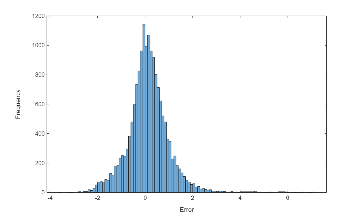
Evaluate the mean squared error (MSE) between the test predictions and the test targets.
err = mean((UTest-TTest).^2,"all")err = single
0.8002
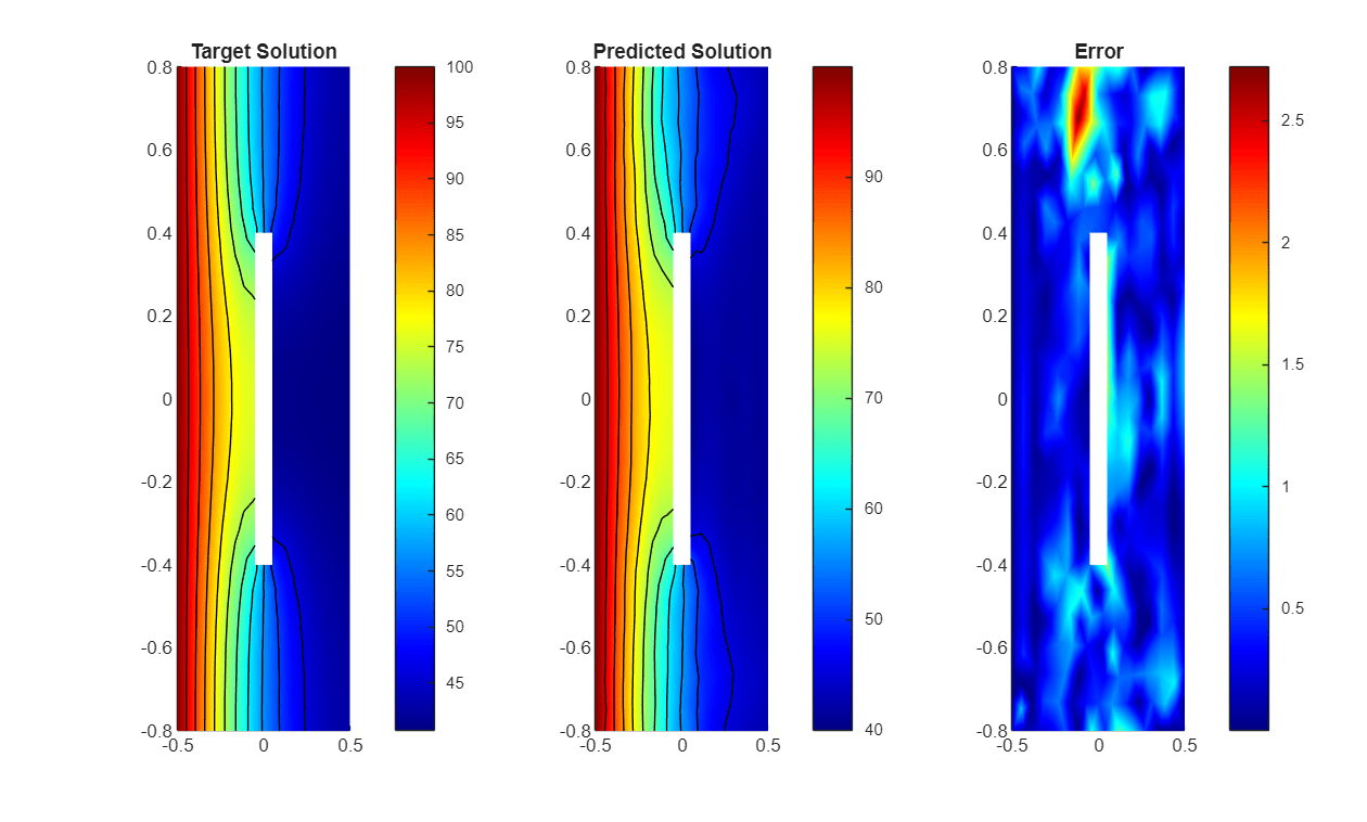
Visualize one of the test predictions in a heat map.
figure
tiledlayout(1,3)
nexttile
pdeplot(thermalmodel.Mesh, ...
    XYData=TTest(:,1,1), ...
    Contour="on", ...
    ColorMap="jet");
title("Target Solution")

nexttile
pdeplot(thermalmodel.Mesh, ...
    XYData=UTest(:,1,1), ...
    Contour="on", ...
    ColorMap="jet");
title("Predicted Solution")

nexttile
pdeplot(thermalmodel.Mesh, ...
    XYData=(abs(UTest(:,1,1)-TTest(:,1,1))), ...
    Contour="off", ...
    ColorMap="jet");
title("Error")
See Also
femodel | dlarray (Deep Learning Toolbox) | dlfeval (Deep Learning Toolbox) | dlgradient (Deep Learning Toolbox) | adamupdate (Deep Learning Toolbox)
Topics
- Solve Poisson Equation on Unit Disk Using Physics-Informed Neural Networks
- Solve PDE Using Fourier Neural Operator (Deep Learning Toolbox)
- Solve PDE Using Physics-Informed Neural Network (Deep Learning Toolbox)