Using Antenna Toolbox with Phased Array Systems
R2026bWhen you create antenna arrays such as a uniform linear array (ULA), you can use antennas that are built into Phased Array System Toolbox™. Alternatively, you can use Antenna Toolbox™ antennas. Antenna Toolbox antennas provide realistic models of physical antennas. They are designed using method of moments. Phased array antennas represent more idealized antennas that are useful for radar performance analysis and higher level modeling. Some phased array antennas cannot be physically realized, such as the isotropic antenna but are still conceptually useful. You can build and analyze systems using both types of antennas in an identical manner. This example shows how to construct a phased array with either Phased Array System Toolbox or Antenna Toolbox antennas.
When you use an Antenna Toolbox antenna in a Phased Array System Toolbox System object™, the antenna response will be normalized by the maximum value of the antenna output over all directions. The maximum value is obtained by finding the maximum of the antenna pattern sampled every five degrees in azimuth and elevation.
Construct ULA of Crossed-Dipole Antennas from Phased Array System Toolbox
Start by creating a ULA of crossed-dipole antennas from Phased Array System Toolbox. Crossed-dipole antennas are used to produce circularly-polarized signals. In this case, set the operating frequency to 2 GHZ and draw the power pattern. Use the pattern method of the phased.CrossedDipoleAntennaElement System object.
fc = 2.0e9;
crosseddipoleantenna = phased.CrossedDipoleAntennaElement(FrequencyRange=[500,2500]*1e6);
pattern(crosseddipoleantenna,fc,[-180:180],0,...
    Type='powerdb')
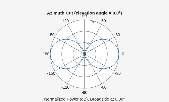
The main axis of this antenna points along the x-axis.
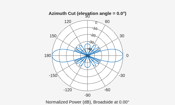
Then, create an 11-element ULA array of crossed-dipole antennas. Specify the element spacing to be 0.4 wavelengths. Taper the array using a Taylor window. Then, draw the array pattern as a function of azimuth at 0 degrees elevation. Use the pattern method of the phased.ULA System object.
c = physconst("LightSpeed");
elemspacing = 0.4*c/fc;
nElements = 11;
array1 = phased.ULA(Element=crosseddipoleantenna,NumElements=nElements,...
    ElementSpacing=elemspacing,Taper=taylorwin(nElements)');
pattern(array1,fc,[-180:180],0,PropagationSpeed=c,...
        Type='powerdb')
Construct ULA of Helix Antennas from Antenna Toolbox
Next, create a uniform linear array (ULA) using the helix antenna from Antenna Toolbox. Helix antennas also produce circularly polarized radiation. Helix antennas are created using the helix function.
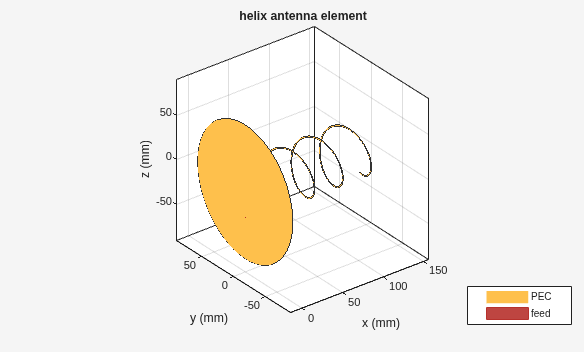
First, specify a 4-turn helix antenna having a 28.0 mm radius and 1.2 mm width. The TiltAxis and Tilt properties let you orient the antenna with respect to the local coordinate system. In this example, orient the main response axis (MRA) along the x -axis to coincide with the MRA of the cross-dipole main axis. By default, the MRA of the antenna points in the z -direction. Rotate the MRA around the y -axis by 90 degrees.
radius = 0.028;
width = 1.2e-3;
nturns = 4;
helixantenna = helix(Radius=radius,Width=width,Turns=nturns,...
    TiltAxis=[0,1,0],Tilt=90);
You can view the shape of the helix antenna using the show function from Antenna Toolbox.
show(helixantenna)
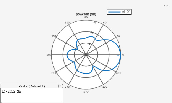
Then, draw the azimuth antenna pattern at 0 degrees elevation at the operating frequency of 2 GHz. Use the pattern function from Antenna Toolbox.
pattern(helixantenna,fc,[-180:180],0,...
    Type='powerdb')
Next, construct an 11-element tapered uniform linear array of helix antennas with elements spaced at 0.4 wavelengths. Taper the array with a Taylor window. You can use the same phased.ULA System object from Phased Array System Toolbox to create this array.
array2 = phased.ULA(Element=helixantenna,NumElements=nElements,...
    ElementSpacing=elemspacing,Taper=taylorwin(nElements)');
Plot the array pattern as a function of azimuth using the ULA pattern method which has the same syntax as the Antenna Toolbox pattern function.
pattern(array2,fc,[-180:180],0,PropagationSpeed=c,...
        Type='powerdb')
Compare Patterns
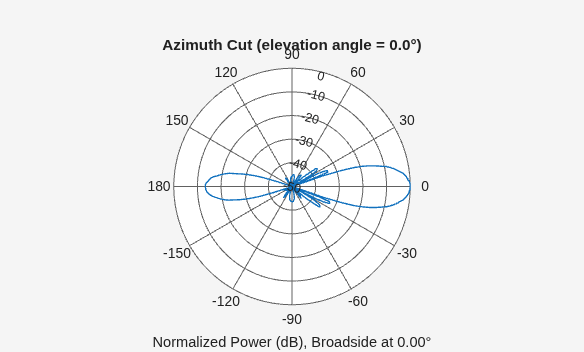
Comparing the two array patterns shows that they are similar along the mainlobe. The backlobe of the helix antenna array pattern is almost 15 dB smaller than that of the crossed-dipole array. This is due to the presence of the ground plane of the helix antenna which reduces backlobe transmission.
Export Conformal Array from Antenna Toolbox
Design a planar phased array of rectangular microstrip patch elements operating at X-band (10 GHz) for a gain of 25 dBi while steering the main beam to 25 degrees. Rectangular patches are chosen for their low profile, ease of fabrication on standard PCB substrates, and natural compatibility with corporate or series feed networks.
To create a phased array with the required input design parameters, use the phasedArrayCalculator object from Antenna Toolbox.
freq=10e9;
p = phasedArrayCalculator(ArrayGain=25,ScanAngle=25,RadiatingElement="rectanglepatch");
Compute the array parameters for the specified operating frequency.
[~] = solve(p,freq);
The calculator uses analytical aperture-based approximations, producing a sinc-shaped radiation pattern for rectangular apertures.
[~,dir_pat1] = plotDirectivity(p,Type="patterns",Frequency=freq);To export the array as a phased.ConformalArray object, use the createArray function with its Type argument set to "phased".
phased_ant = createArray(p,freq,Type="phased")phased_ant =
phased.ConformalArray with properties:
Element: [1×1 patchMicrostrip]
ElementPosition: [3×36 double]
ElementNormal: [2×1 double]
Taper: 1
Evaluate the elevation-cut pattern from the phased array model over a ±50° field of view around boresight (90° elevation).
dir_pat2=patternElevation(phased_ant,freq,0,Elevation=linspace(40,140,200));
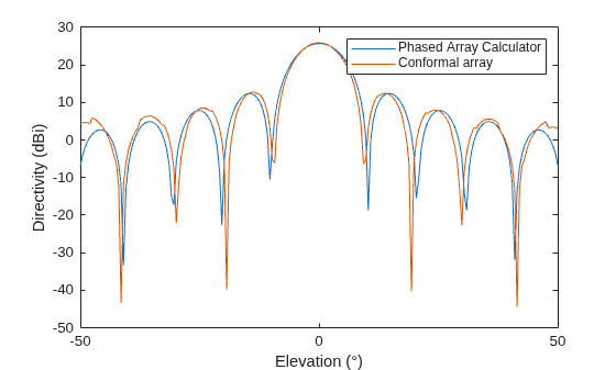
Compare the patterns from the calculator Vs Conformal array.
el = linspace(-50,50,200);
figure;
plot(el,dir_pat1(floor(linspace(1,1001,numel(el)))));
hold on;
plot(el,fliplr(dir_pat2));
legend("Phased Array Calculator","Conformal array");
xlabel("Elevation (°)");
ylabel("Directivity (dBi)");
Construct ULA of measuredAntenna from Antenna Toolbox
Create a uniform linear array (ULA) using the measuredAntenna from Antenna Toolbox. Unlike idealized antenna models, measuredAntenna allows you to import and use realistic antenna electric field (E-field) data obtained from electromagnetic (EM) simulation software (such as ANSYS® HFSS™ or CST Studio Suite®) or from physical measurements in phased array analysis.
First, to create the measuredAntenna object, load the E-field data (frequency, azimuth, elevation and radius) from the antenna_Efield.mat file. Assign these values to the corresponding properties of the measuredAntenna. The Direction property defines the spherical coordinates of observation points over which the field data is specified. It is expressed as a set of azimuth, elevation, and radius values.
data = load("antenna_Efield.mat","E","freq","az","el","R");

Direction = [data.az(:) data.el(:) data.R*ones(numel(data.az),1)];

mesAnt = measuredAntenna(...
    E = data.E, ...
    Direction = Direction, ...
    Azimuth = unique(data.az), ...
    Elevation = unique(data.el), ...
    FieldFrequency = data.freq, ...
    PhaseCenter = [0 0 0], ...
    NumPorts = 1);
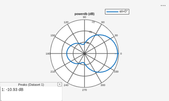
Then, plot the azimuth radiation antenna pattern at 0° elevation and an operating frequency of 2 GHz using the pattern function from Antenna Toolbox.
figure
pattern(mesAnt,data.freq,-180:5:180,0,...
    Type = 'powerdb')
Next, construct an 11-element tapered ULA using the measuredAntenna object with elements spaced at 0.4 wavelengths. Apply a Taylor window to taper the array. You can use the same phased.ULA System object from Phased Array System Toolbox to create this array.
array3 = phased.ULA(Element = mesAnt,NumElements = nElements,...
    ElementSpacing = elemspacing,Taper = taylorwin(nElements)');
Finally, plot the array radiation pattern as a function of azimuth angle using the pattern function of the ULA which has a syntax similar to Antenna Toolbox pattern function.
pattern(array3,data.freq,-180:180,0,PropagationSpeed = c,...
    Type = 'powerdb')
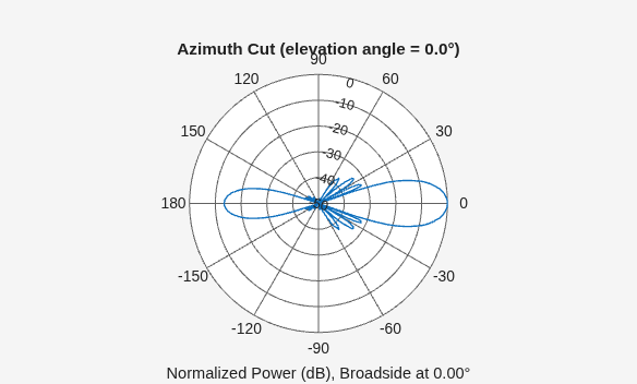
Using measuredAntenna, you can move beyond idealized antenna assumptions and develop phased array models that more accurately reflect real-world deployment scenarios.

