Create DQN Agent Using Deep Network Designer and Train Using Image Observations

R2026b

This example shows how to create a deep Q-learning network (DQN) agent that can swing up and balance a pendulum modeled in MATLAB®. In this example, you create the DQN agent using Deep Network Designer. For more information on DQN agents, see Deep Q-Network (DQN) Agent.

Pendulum Swing-Up with Image MATLAB Environment

The reinforcement learning environment for this example is a simple frictionless pendulum that initially hangs in a downward position. The training goal is to make the pendulum stand upright using minimal control effort.

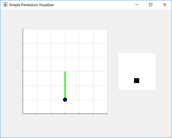
For this environment:

• The upward balanced pendulum position is zero radians, and the downward hanging position is pi radians.

• The torque action signal from the agent to the environment can take any of the five possible integer values from –2 to 2 N·m (counterclockwise positive).

• The observations from the environment are the simplified grayscale image of the pendulum and the pendulum angle derivative.

• The reward $r_t$, which the environment provides to the agent at every time step, is

$$r_t=-\left({{\theta }_t}^2+0.1{\underset{}{\overset{\dot{}}{{\theta }_t}}}^2+0.001u_{t-1}^2\right)$$

Here:

• ${\theta }_t$ is the angle of displacement from the upright position (counterclockwise positive).

• $\underset{}{\overset{\dot{}}{{\theta }_t}}$ is the derivative of the displacement angle.

• $u_{t-1}$ is the control effort from the previous time step.

For more information on the continuous action space version of this model, see Train DDPG Agent with Custom Networks Using Image Observation.

Specify Random Number Stream Seed and Algorithm for Reproducibility

Some sections in this example require random number computations. Specify the seed and random number generator algorithm at the beginning of a section to use the same random number sequence each time you run it. Preserving the random number sequence allows you to reproduce the results of the section. For more information, see Results Reproducibility.

Set the random number seed to 0 and the algorithm to Mersenne Twister. For more information, see rng.

previousRngState = rng(0,"twister");

The output previousRngState is a structure that contains information about the previous state of the sequence. You will restore the state at the end of the example.

Create Environment Object

Create a predefined environment object for the pendulum.

env = rlPredefinedEnv("SimplePendulumWithImage-Discrete");

The interface has two observations. The first observation, named "pendImage", is a 50-by-50 grayscale image.

obsInfo = getObservationInfo(env);
obsInfo(1)

ans = 
  rlNumericSpec with properties:

     LowerLimit: 0
     UpperLimit: 1
           Name: "pendImage"
    Description: [0×0 string]
      Dimension: [50 50]
       DataType: "double"

The second observation, named "angularRate", is the angular velocity of the pendulum.

obsInfo(2)

ans = 
  rlNumericSpec with properties:

     LowerLimit: -Inf
     UpperLimit: Inf
           Name: "angularRate"
    Description: [0×0 string]
      Dimension: [1 1]
       DataType: "double"

The interface has a discrete action space where the agent can apply one of five possible torque values to the pendulum: –2, –1, 0, 1, or 2 N·m.

actInfo = getActionInfo(env)

actInfo = 
  rlFiniteSetSpec with properties:

       Elements: [-2 -1 0 1 2]
           Name: "torque"
    Description: [0×0 string]
      Dimension: [1 1]
       DataType: "double"

Construct Critic Network Using Deep Network Designer

DQN agents use a parameterized Q-value function approximator to estimate the value of the policy. Because a DQN agent has a discrete action space, you can use a vector (that is, multi-output) Q-value function critic, which is generally more efficient than a comparable single-output critic. However, for this example, use a standard single-output Q-value function critic.

To model the parameterized Q-value function within the critic, use a neural network with three input layers (two for the observation channels, as specified by obsInfo, and the other for the action channel, as specified by actInfo) and one output layer (which returns the scalar value). For more information on creating Q-value function approximators based on a deep neural network, see Create Actors, Critics, and Policy Objects.

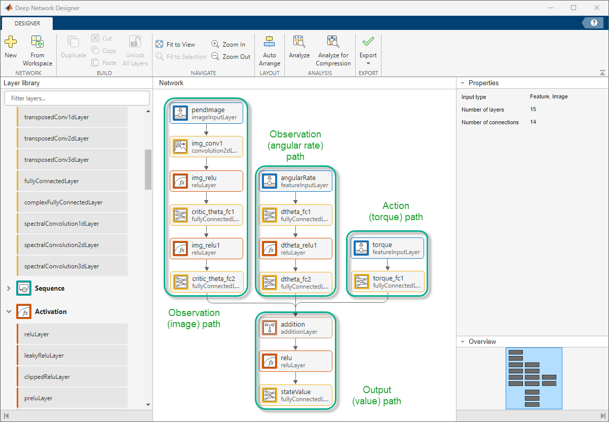
Construct the critic network interactively by using the Deep Network Designer app. To launch the app, you can type at deepNetworkDesigner the MATLAB® command window. To build the network, first select the Blank Network (New) page, then create separate input paths for each observation and action. These paths learn lower-level features from their respective inputs. Then create a common output path that combines the outputs from the input paths.

Create Image Observation Path

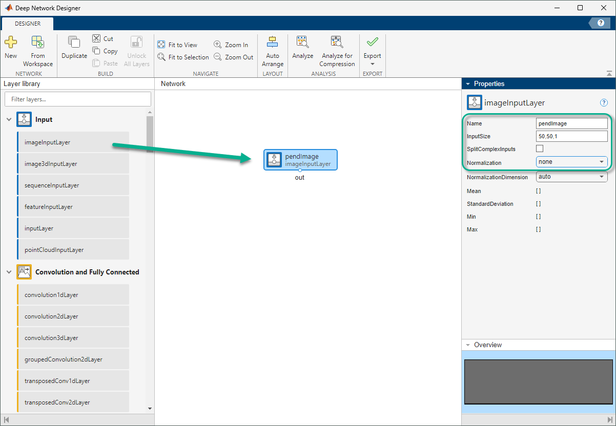
To create the image observation path, first drag an imageInputLayer from the Layer Library pane to the canvas. Set the layer Name to pendImage, the layer InputSize to 50,50,1 for the image observation, and set Normalization to none.

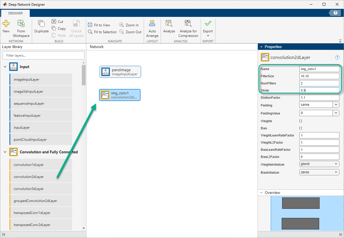
Second, drag a convolution2DLayer to the canvas and connect the input of this layer to the output of the imageInputLayer. Create a convolution layer with 2 filters (NumFilters property) that have a height and width of 10 (FilterSize property), and use a stride of 5 in the horizontal and vertical directions (Stride property). Set the layer Name to img_conv1.

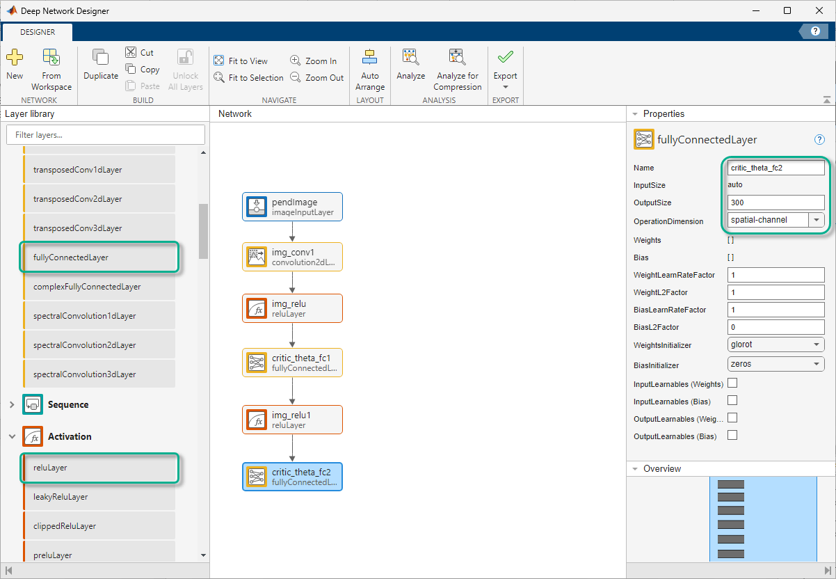
Finally, complete the image path network with two sets of reLULayer and fullyConnectedLayer layers. Set the output sizes of the first and second fullyConnectedLayer layers to 400 and 300, respectively. Name the layers as in the figure. Connect all the layers.

Create All Input Paths and Output Path

Construct the other input paths and the output path in a similar manner. For this example, use the following options.

Angular rate path (scalar input):

• featureInputLayer — Set InputSize to 1 and Normalization to none.

• fullyConnectedLayer — Set OutputSize to 400.

• reLULayer

• fullyConnectedLayer — Set OutputSize to 300.

Action (torque) path (scalar input):

• featureInputLayer — Set InputSize to 1 and Normalization to none.

• fullyConnectedLayer — Set OutputSize to 300.

Output path:

• additionLayer — Connect the output of all input paths to the input of this layer.

• reLULayer

• fullyConnectedLayer — Set OutputSize to 1 for the scalar value function.

Connect the paths.

Export Network from Deep Network Designer

To export the network to the MATLAB workspace, in Deep Network Designer, click Export. Deep Network Designer exports the network as a new variable containing the network layers. You can create the critic representation using this layer network variable.

Alternatively, to generate equivalent MATLAB code for the network, click Export > Generate Network Code Without Parameters.

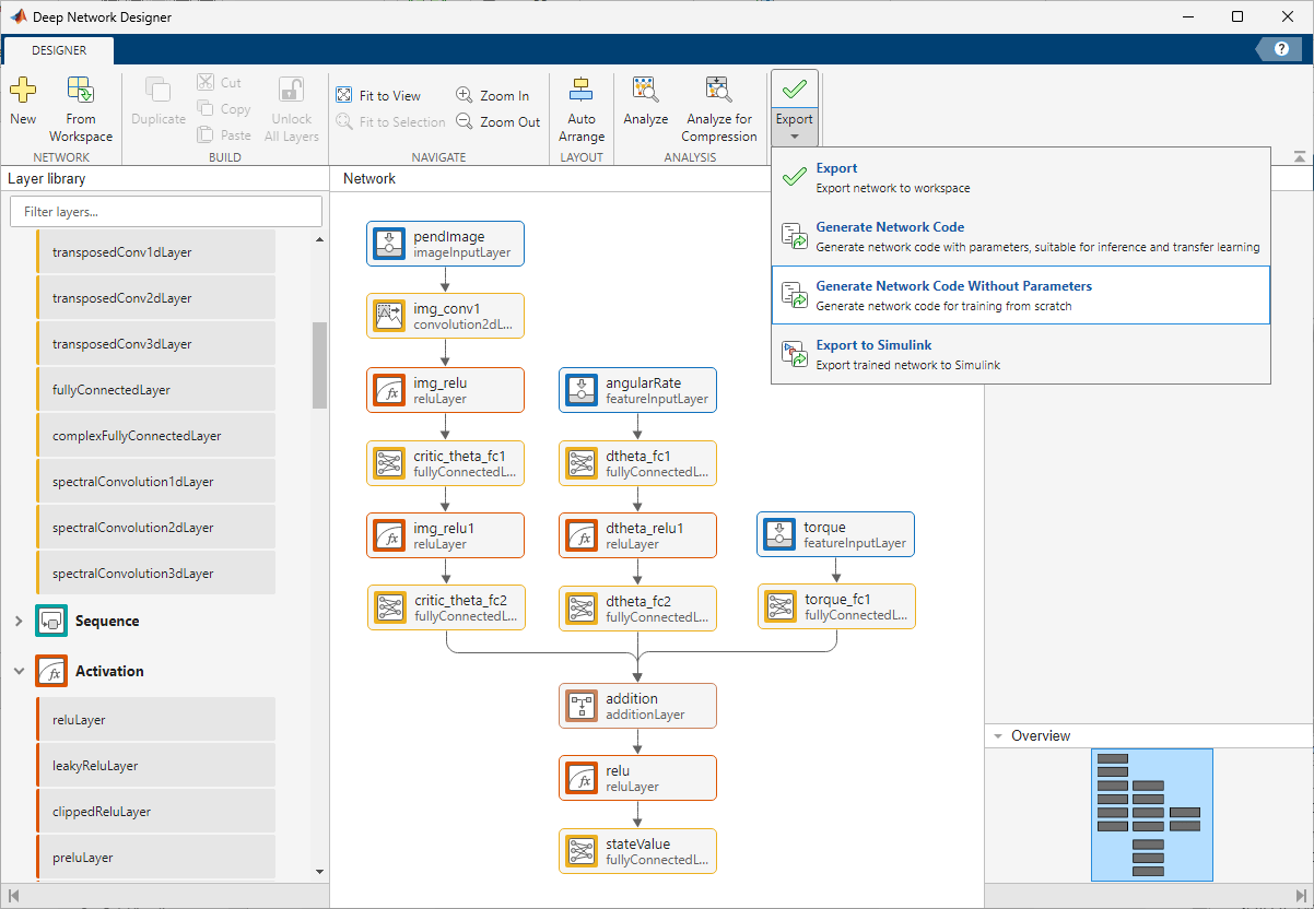
Deep Network Designer creates a new script that builds the network object. The generated code is as follows.

Generated Code

Create an empty dlnetwork object.

net = dlnetwork;

Add branches to the dlnetwork. Each branch is a linear array of layers.

tempNet = [
    imageInputLayer([50 50 1],"Name","pendImage","Normalization","none")
    convolution2dLayer([10 10],2,"Name","img_conv1","Padding","same","Stride",[5 5])
    reluLayer("Name","img_relu")
    fullyConnectedLayer(400,"Name","critic_theta_fc1")
    reluLayer("Name","img_relu1")
    fullyConnectedLayer(300,"Name","critic_theta_fc2")];
net = addLayers(net,tempNet);

tempNet = [
    featureInputLayer(1,"Name","angularRate")
    fullyConnectedLayer(400,"Name","dtheta_fc1")
    reluLayer("Name","dtheta_relu1")
    fullyConnectedLayer(300,"Name","dtheta_fc2")];
net = addLayers(net,tempNet);

tempNet = [
    featureInputLayer(1,"Name","torque")
    fullyConnectedLayer(300,"Name","torque_fc1")];
net = addLayers(net,tempNet);

tempNet = [
    additionLayer(3,"Name","addition")
    reluLayer("Name","relu")
    fullyConnectedLayer(1,"Name","stateValue")];
net = addLayers(net,tempNet);

% Clean up helper variable.
clear tempNet;

Connect all the branches of the network to create the network graph.

net = connectLayers(net,"critic_theta_fc2","addition/in1");
net = connectLayers(net,"torque_fc1","addition/in3");
net = connectLayers(net,"dtheta_fc2","addition/in2");
net = initialize(net);

View the critic network configuration.

figure
plot(net)

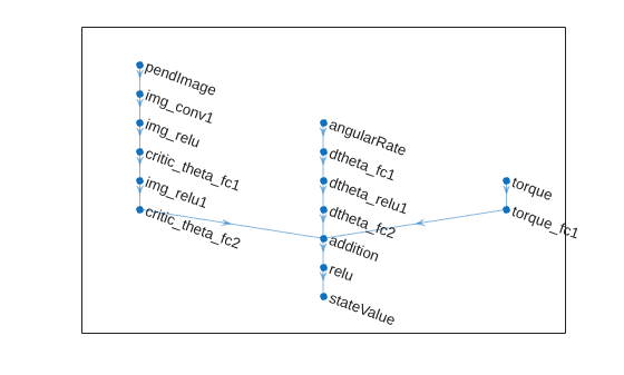
Initialize the dlnetwork object and display the number of parameters.

net = initialize(net);
summary(net)

   Initialized: true

   Number of learnables: 322.9k

   Inputs:
      1   'pendImage'     50×50×1 images
      2   'angularRate'   1 features
      3   'torque'        1 features

Create the critic using the neural network, the action and observation specifications, and the names of the input layers to be connected to the observations and action channels. For more information, see rlQValueFunction.

critic = rlQValueFunction(net,obsInfo,actInfo, ...
    "ObservationInputNames",["pendImage","angularRate"], ...
    "ActionInputNames","torque");

Specify options for the critic using rlOptimizerOptions.

criticOpts = rlOptimizerOptions(LearnRate=1e-03,GradientThreshold=1);

Specify the DQN agent options using rlDQNAgentOptions. Include the training options for the actor and critic.

agentOpts = rlDQNAgentOptions( ...
    UseDoubleDQN=false, ...    
    CriticOptimizerOptions=criticOpts, ...
    ExperienceBufferLength=1e6, ... 
    SampleTime=env.Ts);

You can also set or modify agent options using dot notation.

agentOpts.EpsilonGreedyExploration.EpsilonDecay = 1e-5;

Alternatively, you can create the agent first, and then modify its options using dot notation.

Create the DQN agent using the critic and the agent options object. For more information, see rlDQNAgent.

agent = rlDQNAgent(critic,agentOpts);

Train DQN Agent

To train the agent, first specify the training options. For this example, use the following options.

• Run each training for a maximum of 5000 episodes, with each episode lasting a maximum of 500 time steps.

• Display the training progress in the Episode Manager dialog box (set the Plots option to "training-progress").

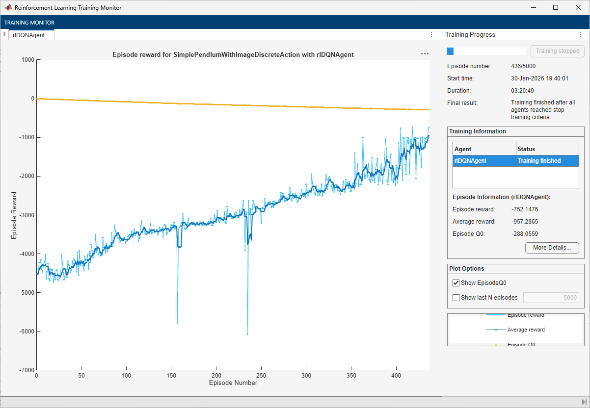
• Disable the command line display (set the Verbose option to false).

• Stop the training when the agent receives an average cumulative reward greater than –1000 over the default window length of five consecutive episodes. At this point, the agent can quickly balance the pendulum in the upright position using minimal control effort.

For more information on training options, see rlTrainingOptions.

trainOpts = rlTrainingOptions( ...
    MaxEpisodes=5000, ...
    MaxStepsPerEpisode=500, ...
    Verbose=false, ...
    Plots="training-progress", ...
    StopTrainingCriteria="AverageReward", ...
    StopTrainingValue=-1000);

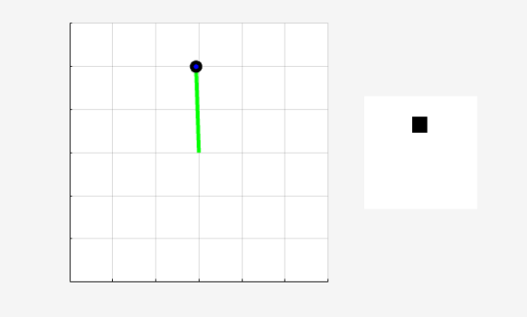
Visualize the pendulum system during training or simulation using the plot function.

plot(env)

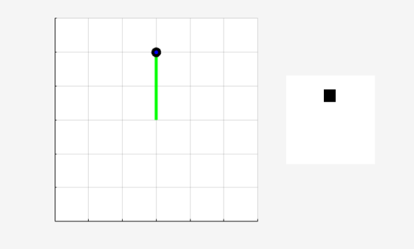
Train the agent using the train function. Training is a computationally intensive process that might take several hours to complete. To save time, load a pretrained agent by setting doTraining to false. To train the agent yourself, set doTraining to true.

doTraining = false;
if doTraining
    % Train the agent.
    trainingStats = train(agent,env,trainOpts);
else
    % Load pretrained agent for the example.
    load("MATLABPendImageDQN.mat","agent");
end

Simulate Trained Agent

To validate the performance of the trained agent, simulate it within the pendulum environment. For more information on agent simulation, see rlSimulationOptions and sim.

simOptions = rlSimulationOptions(MaxSteps=500);
experience = sim(env,agent,simOptions);

totalReward = sum(experience.Reward)

totalReward = 
-767.5060

Restore the random number stream using the information stored in previousRngState.

rng(previousRngState);