Comparison of Lumped and Distributed EM Models for Low Pass Filters

This example shows how to compare lumped and distributed electromagnetic (EM) model for low pass filters.

1. Use an rffilter object from the RF Toolbox to create a lumped element implementation for the low pass filter.

2. Use Richards and Kurodas identities to convert the lumped element filter into distributed element filter by calculating the line impedances.

3. Use the microstripLine design function to calculate the length and width of the transmission lines having different impedance

4. Use the filterStub catalog in RF PCB Toolbox is used to create and analyze this filter.

You will observe that the results from the RF Toolbox and RF PCB Toolbox are matching very well.

Define Frequencies

designFreq = 4e9;
freqRange = linspace(1e9,2*designFreq,51); 

Create RF Filter

Use rffilter object to create an RF filter with a filterOrder 3 and with a 3 dB equal ripple passband response.

filt = rffilter('FilterOrder',3,'FilterType','Chebyshev');
filt.PassbandFrequency = designFreq;
filt.PassbandAttenuation = 2;

Use the sparameters function to compute the S-Parameters of the low pass filter and plot them using the rfplot function.

spar = sparameters(filt,linspace(1e9,8e9,101));
figure,rfplot(spar);

The rffilter computes the values of L and C for the required response. You can access these values from the DesignData property of the RF filter.

filt.DesignData

ans = struct with fields:
            FilterOrder: 3
              Inductors: [5.3927e-09 5.3927e-09]
             Capacitors: 6.6261e-13
               Topology: 'lclowpasstee'
      PassbandFrequency: 4.0000e+09
    PassbandAttenuation: 2

Transform the L and C values into normalized low pass filter element values. In order to construct the distributed form of this filter, you need to convert the lumped elements into distributed transmissions lines using Richards transformations and Kuroda identities. Using these g1, g2 and g3 values compute the line impedances for the series lines and the open stubs

L = filt.DesignData.Inductors;
C = filt.DesignData.Capacitors;

% Computation
% normalized low-pass element values
g1 = 2*pi*filt.PassbandFrequency*L(1)/filt.Zin;
g3 = g1;
g2 = 2*pi*filt.PassbandFrequency*C*filt.Zin;

% Richard's transformation and Kuroda's 2nd identity
n2 = 1+(1/g1);
Zshunt1 = n2*filt.Zin;
Zseries1 = n2*g1*filt.Zin;
Zshunt2 = (1/g2)*filt.Zin;
Zseries2 = n2*g3*filt.Zin; %#ok<*NASGU>
Zshunt3 = n2*filt.Zin;

After calculating the impedances of transmission lines, use the design function from the microstripLine catalog to calculate the lengths and widths of the respective impedance.

obj = microstripLine;
portline = design(obj,designFreq,'Z0',50,'LineLength',1/8);
seriesLine1 = design(obj,designFreq,'Z0',Zseries1,'LineLength',1/8);
seriesLine2 = design(obj,designFreq,'Z0',Zseries2,'LineLength',1/8);
stub1 = design(obj,designFreq,'Z0',Zshunt1,'LineLength',1/8);
stub2 = design(obj,designFreq,'Z0',Zshunt2,'LineLength',1/8);
stub3 = design(obj,designFreq,'Z0',Zshunt3,'LineLength',1/8);

Comparison with EM Simulation

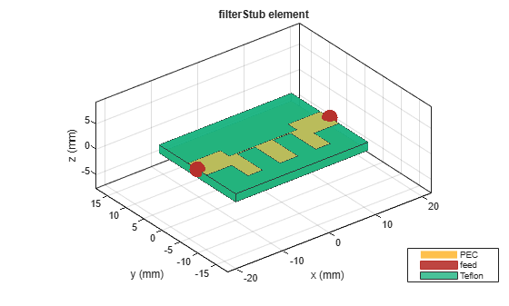
Use the filterStub object and create the filter using the dimensions from the RF filter.

filterEM = filterStub;
filterEM.PortLineLength = portline.Length;
filterEM.PortLineWidth = portline.Width;
filterEM.SeriesLineLength = [seriesLine1.Length seriesLine2.Length];
filterEM.SeriesLineWidth = [seriesLine1.Width seriesLine2.Width];
filterEM.StubLength = [stub1.Length stub2.Length stub3.Length];
filterEM.StubWidth = [stub1.Width stub2.Width stub3.Width];
filterEM.StubDirection = [0 0 0];
filterEM.StubShort = [0 0 0];
filterEM.StubOffsetX= [-seriesLine1.Length 0 seriesLine2.Length];
filterEM.GroundPlaneWidth = max(filterEM.StubLength)*3;
show(filterEM);

Use the mesh function and set the MaxEdgeLength to 5 mm to ensure 15 triangles per wavelength.

figure,mesh(filterEM,'MaxEdgeLength',0.02);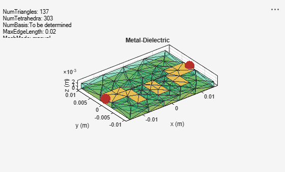

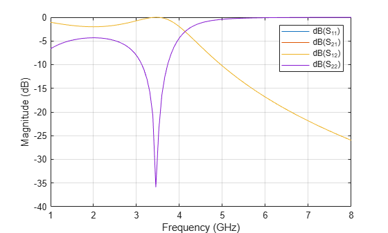
Use the sparameters function to calculate the S-parameters and plot it using the rfplot function.

spar = sparameters(filterEM,linspace(1e9,8e9,51));
figure,rfplot(spar);