Feedback Control of a ROS-Enabled Robot
Use Simulink® to control a simulated robot running in a separate ROS-based simulator.
This example involves a model that implements a simple closed-loop proportional controller. The controller receives location information from a simulated robot (running in a separate ROS-based simulator) and sends velocity commands to drive the robot to a specified location. Adjust parameters while the model is running and observe the effect on the simulated robot.
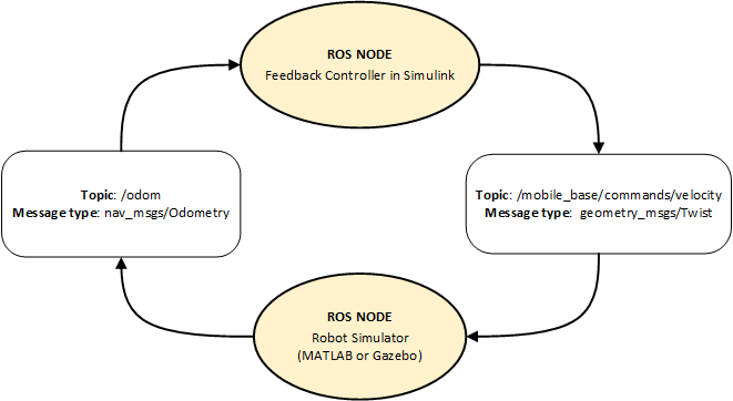
The following figure summarizes the interaction between Simulink and the robot simulator (the arrows in the figure indicate ROS message transmission). The /odom topic conveys location information, and the /mobile_base/commands/velocity topic conveys velocity commands.
Start a Robot Simulator and Configure Simulink
Follow the steps in the Connect to ROS-enabled Robot from Simulink example to do the following:
Start a MATLAB® or Gazebo® robot simulator.
Configure Simulink to connect to the ROS network.
Open Existing Model
After connecting to the ROS network, open the example model.
open_system('robotROSFeedbackControlExample.slx');The model implements a proportional controller for a differential-drive mobile robot. At each time step, the algorithm orients the robot toward the desired location and drives it forward. Once the desired location is reached, the algorithm stops the robot.
open_system('robotROSFeedbackControlExample/Proportional Controller');Note that there are four tunable parameters in the model (indicated by colored blocks).
Desired Position (at top level of model): The desired location in
(X,Y)coordinatesDistance Threshold: The robot stops if it is closer than this distance from the desired location
Linear Velocity: The forward linear velocity of the robot
Gain: The proportional gain when correcting the robot orientation
The model also has a Simulation Rate Control block (at top level of model). This block ensures that the simulation update intervals follow wall-clock elapsed time.
Run the Model
Run the model and observe the behavior of the robot in the robot simulator.
Position windows on your screen so that you can observe both the Simulink model and the robot simulator.
Click Play to start simulation.
While the simulation is running, double-click the Desired Position block and change the
Constantvalue to[2 3]. Observe that the robot changes its heading.While the simulation is running, open the Proportional Controller subsystem and double-click the Linear Velocity (slider) block. Move the slider to
2. Observe the increase in robot velocity.Click Stop to end the simulation.
Observe Rate of Incoming Messages
Use the MATLAB-based simulator to observe the timing and rate of incoming messages.
Close any existing Robot Simulator figure windows.
Click Play to start simulation.
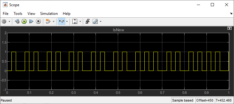
Open the Scope block. Observe that the
IsNewoutput of the Subscribe block is always0, indicating that no messages are being received for the/odomtopic. The horizontal axis of the plot indicates simulation time in seconds.At the MATLAB command line, type
ExampleHelperSimulinkRobotROSto start the MATLAB-based robot simulator. This simulator publishes/odommessages at approximately20Hz in wall-clock elapsed time.In the Scope display, observe that the IsNew output has the value
1at an approximate rate of20times per second, in elapsed wall-clock time.
The synchronization with wall-clock time is due to the Simulation Rate Control block. Typically, a Simulink simulation executes in a free-running loop whose speed depends on complexity of the model and computer speed (see Simulation Loop Phase (Simulink)). The Simulation Rate Control block attempts to regulate Simulink execution so that each update takes 0.02 seconds in wall-clock time when possible. (This is equal to the fundamental sample time of the model.) See the comments inside the block for more information.
In addition, the Enabled subsystems for the Proportional Controller and the Command Velocity Publisher ensure that the model only reacts to genuinely new messages. If enabled subsystems were not used, the model would repeatedly process the same (most-recently received) message repeatedly, leading to wasteful processing and redundant publishing of command messages.