Define Step Size and Number of Nonlinear Iterations for Simscape Real-Time Simulation
This example shows you how to configure a Simscape™ model for real-time simulation by adjusting the step size and nonlinear iterations. Real-time targets use fixed-step and fixed-cost simulation, which means that each time step is the same length and consumes the same computational resources. By default, Simscape models use variable-step simulation, where the solver adapts the step size and computational resources.
To prepare a model for real-time simulation, you first determine that your model is stable and accurate in variable-step simulation. Then, use the variable-step results to estimate the step size and number of nonlinear iterations for fixed-step and fixed-cost simulation. Next, adjust the step size and number of nonlinear iterations to find an acceptable balance between accuracy and execution speed. This chart illustrates the process that you take to configure your model.
In this example, you configure a Simscape model of a mechanical system to run in fixed-step and fixed-cost simulation. To improve the simulation results and reduce the computational cost, you adjust the step size and the number of nonlinear iterations and compare the results to the variable-step simulation data.
Gather Variable-Step Simulation Results
Open the MechanicalSystemWithTranslationFriction model.
openExample("simscape/MechanicalSystemWithTranslationalFrictionExample")This model uses variable-step simulation. To convert the model to fixed-step size, first identify the step size that the variable-step simulation uses by using the Solver Profiler. In the Debug tab, in the Performance section, click Performance > Solver Profiler. The Solver Profiler opens.
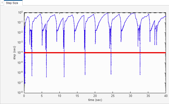
Simulate the model in the Solver Profiler. In the Profile section, click Run. The Solver Profiler populates the Step Size tab with a plot of step size in seconds versus simulation time. The Solver Profiler also indicates issues that the model has in the Suggestion, Solver Exception, and Solver Reset tabs in the bottom pane. If your model contains issues in variable-step simulation, resolve them before configuring your model for fixed-step and fixed-cost simulation. In this example, the Solver Profiler does not report issues.
Estimate the Step Size
To identify an initial step size for fixed-step and fixed-cost simulation,
estimate the simulation step size. In this example, the solver uses step sizes above
0.0001 for most of the simulation. When the step size
decreases below this value, the solver quickly increases the step size above
0.0001.
Test and Update the Step Size
To test your model in fixed-step and fixed-cost simulation, capture data from the variable-size step model to use as a baseline. Then put the model in fixed-step and fixed-cost mode, run the model again, and compare the data between the two simulations.
To capture the simulation data, you can either log the signals and view the data in
the Simulation Data Inspector, or retrieve the Simscape data programmatically by using the sim function. In
this example, log the displacement into the Simulation Data Inspector.
Right-click the input signal to the Displacement block, and in the
Log Signals row, click the Log Signals button
.
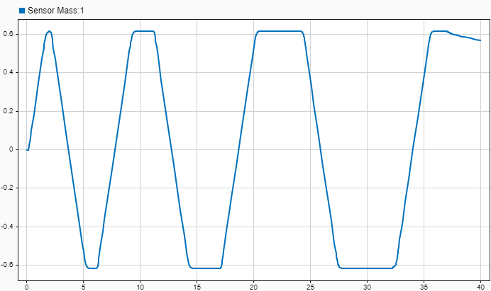
Simulate the data in variable-step. To view the data, open the Simulation Data Inspector. In the model, in the Simulation tab, in the Review Results section, click Data Inspector. The Simulation Data Inspector opens and displays the logged data.
Next, prepare the model for fixed-step and fixed-cost simulation.
In the model, open the
Velocity Inputsubsystem.Double-click the Solver Configuration block. The Block Parameters window opens.
Enable the Use local solver parameter. This parameter enables the Sample time and Solver type parameters.
Enable the Use fixed-cost runtime consistency iterations parameter. This parameter enables the Nonlinear iterations, Computer impulses, and Maximum threads for function evaluation parameters.
Simulate the model with the default Solver Configuration block settings and view the results in the Simulink Data Inspector.
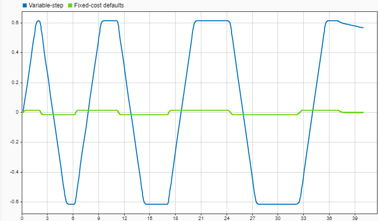
The results show that the fixed-step and fixed-cost results do not match the variable-step results. To adjust the simulation results, you must adjust the Solver Configuration block settings.
Adjust Simulation Settings
To improve the results, decrease the step size. In the Solver
Configuration block, set Step size to
0.0001 and rerun the simulation.
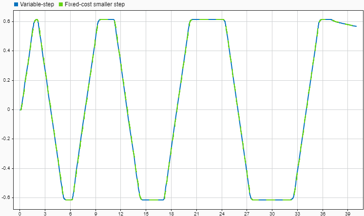
After decreasing the step size, the simulation takes longer to run. In some circumstances, your hardware may not support the additional computational requirements when you decrease the step size.
Although the results appear to match, you can quantitatively compare them in the Simulation Data Inspector.
In the Simulation Data Inspector, click Compare.
Set the Baseline property to the variable-step simulation results.
Set the Compare to property to the fixed-step and fixed-cost simulation results.
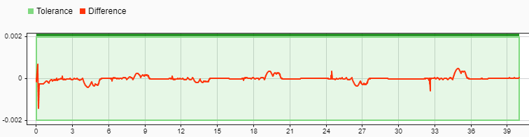
Expand the Options button to the right of the Compare to property and set the absolute tolerance by setting Absolute to
0.002.Click Compare.
The Simulation Data Inspector displays the differences between
the data in a plot. In this example, the difference between the fixed-cost simulation
and the variable-step simulation does not exceed a magnitude of
0.002.
Reduce Nonlinear Iterations
Fixed-step and fixed-cost models run may more slowly than variable-step models. To improve the computational performance, you can increase the step size or reduce the number of nonlinear iterations. To reduce the nonlinear iterations and test the results.
Open the Solver Configuration block in the
Velocity Inputsubsystem.Change the Nonlinear iterations parameter value to
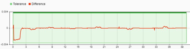
1.Expand the Options button to the right of the Compare to property and set the absolute tolerance by setting Absolute to
0.004.Simulate the model and compare the results.
In this example, the difference is larger than in the previous
simulation, but it does not exceed a magnitude of 0.004.
When you find a combination of solver settings that provides accurate enough results and a simulation speed that is less than your execution-time budget, you can run your model on a real-time target machine.
Modify Model Outside of Fixed-Cost and Fixed-Step Parameters
Sometimes, decreasing the step size and increasing the number of nonlinear iterations is not be possible in your model due to hardware requirements, and increasing the step size and decreasing the number of nonlinear iterations can produce results that differ too much from the variable-step results. If you cannot find an acceptable step size and number of nonlinear iterations, you can improve simulation speed and accuracy by modifying the scope or fidelity of your model. If you cannot make your model real-time capable by changing the scope or fidelity of your model, increase your real-time computing capability. For more information, see Simulating Parts of the System in Parallel.
See Also
Solver
Profiler | simscape.getLocalSolverFixedCostInfo