Use Scaling by Nominal Values to Improve Performance
Nominal values provide a way to specify the expected magnitude of a variable in a model, similar to specifying a transformer rating, or setting a range on a voltmeter. This example shows how you can fine-tune scaling of individual variables in a model to improve the solver performance and increase the simulation robustness.
When the solver performs numerical simulation and analysis, it uses variables without units. Nominal values is a way to convert engineering variables with units into variables without units and to scale them for optimal solver performance. The nominal value has a value with a unit and this unit is used to strip away the unit for numerical calculations. The nominal value then determines the magnitude of the variable as seen by the numerical algorithms. It is generally beneficial to have magnitudes of similar scale.
Consider a simple mass-spring-damper model with a large spring constant.
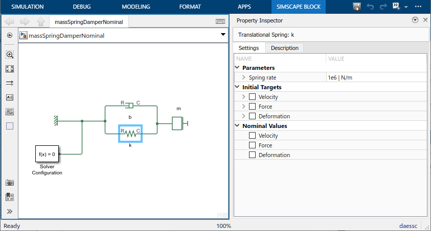
The model uses the default block parameter settings, with the exception of spring rate:
Spring rate, k = 1e6 N/m
Damping coefficient, b = 100 N/(m/s)
Mass, m = 1 kg
The initial mass velocity variable, v, has
High priority and the initial target value of 0.1 m/s. The model
uses the default nominal values, with m as the length unit.
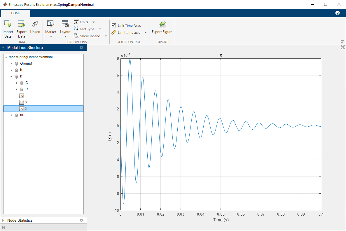
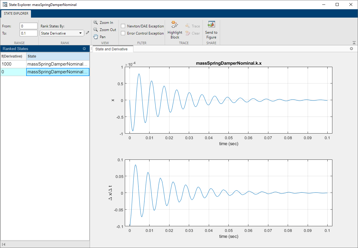
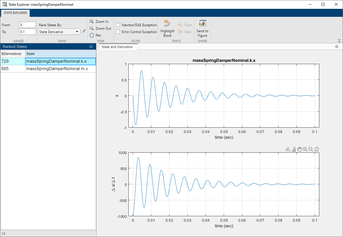
When you simulate this model, the spring Deformation (position) variable x is small, in the 10^-5 m range.
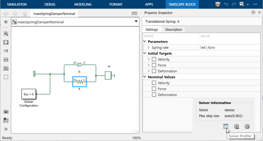
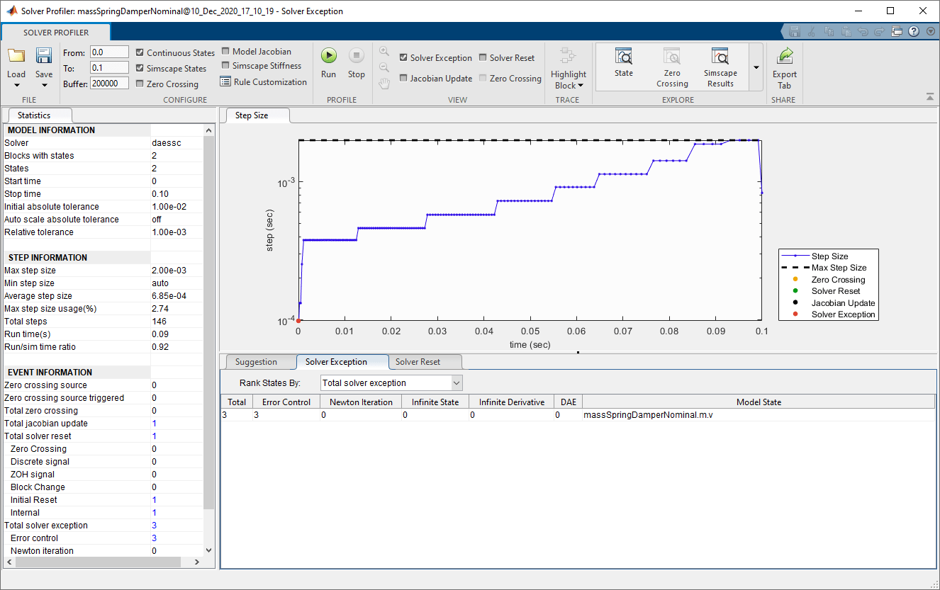
Open the Solver Profiler by clicking the hyperlink in the lower-right corner of the model window.
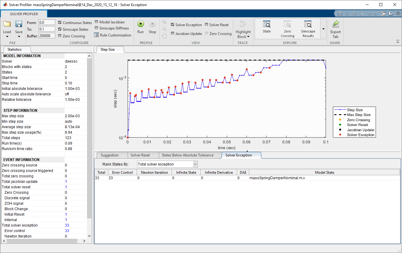
The solver completely ignores the position variable and just looks at the velocity variable. The numerical magnitude of position is below the tolerance for that variable.
The State Viewer, accessed from the Solver Profiler toolstrip, shows the magnitude of each variable as seen by the solvers.
The situation is clear if we look at the model equations:
When k is very large, compared to m and b, then x is small, so that the product k*x is of reasonable size, compared to the other terms in the equation. To remedy the situation, we need to scale x. In other words, we need to choose a nominal value for x that is small, so that the scaled variable, xs, becomes more reasonably sized:
where c is large. For example, if the nominal value is 1 μm and the original x is in m, then c is 1e6. The equations then become:
and the terms have magnitudes of similar scale.
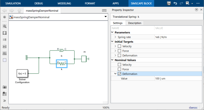
Let us apply this scaling principle to the model variables. First, use the Property
Inspector to change the nominal value of the spring Deformation variable,
x, to 100 um (1e-4 m).
Similarly, change the nominal value of the mass Velocity variable to 10 cm/s (0.1 m/s).
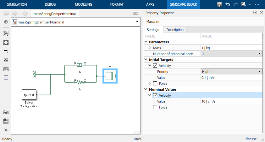
This brings the scale of the magnitude of both variables seen by the solver to approximately 1.
Rerun the simulation.
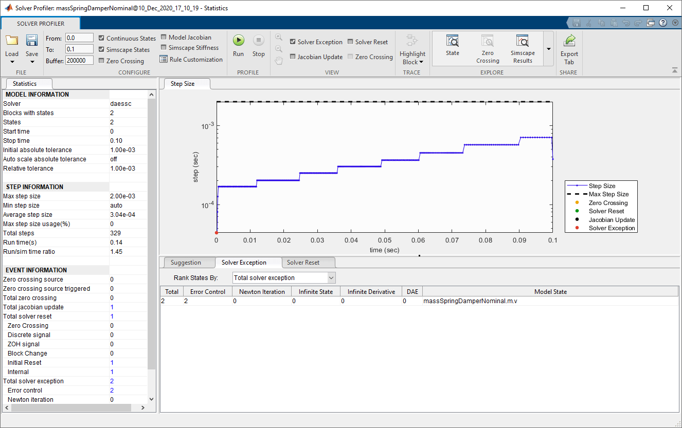
There are now only two solver exceptions, at the beginning of the simulation.
Note that the effective absolute tolerance is now tighter for the mass velocity. The
effective absolute tolerance for Simscape™ models has a unit, and is computed as (nominal value * global
AbsTol without units). In the first simulation run the effective absolute
tolerance was 1e-3 m/s, and now it is 1e-4 m/s because the nominal value changed magnitude and
the global AbsTol is still 1e-3. However, the speed of
the simulation is similar, even with the increased AbsTol on the mass
velocity and increased time steps.
The values, as seen by the solver, are similar in magnitude for both the velocity and position variables.
Now, change the global AbsTol to 1e-2, to more
closely match the accuracy of the velocity variable during the first simulation run.
Rerun the simulation.
The time steps are similar and the number of exceptions is 3, also at the beginning of simulation.