Explore Model Hierarchy

Simulink^® models can be organized into hierarchical components. In a hierarchical model, you can choose to view the system at a high level, or navigate down the model hierarchy to see increasing levels of model detail.

View Model Hierarchy

Open Model

To start, open the smart_braking model.

In the model:

A vehicle moves as the gas pedal is pressed.
A proximity sensor measures the distance between the vehicle and an obstacle.
An alert system generates an alarm based on that proximity.
The alarm automatically controls the brake to prevent a collision.

When you build a model, you connect blocks together to model complex components that represent system dynamics. In this model, Vehicle, Proximity sensor, and Alert system are all complex components with multiple blocks that exist in a hierarchy of subsystems. To view the contents of a subsystem, double-click the subsystem.

To view a representation of the complete model hierarchy, click the Hide/Show Model Browser button at the bottom left corner of the model window.

The Model Browser shows that all subsystems you view at the top level have subsystems of their own. Expand each subsystem node to see the subsystems it contains. You can navigate through the hierarchy in the Model Browser. For example, expand the Proximity sensor node and then select the Sensor model subsystem.

The address bar shows which subsystem you are viewing. To open the subsystem in a separate window, right-click the subsystem and select Open In New Window.

Every input or output port on a subsystem has a corresponding Inport or Outport block inside the subsystem. These blocks represent data transfer between a subsystem and its parent. When a system contains multiple input or output ports, the number on the Inport or Outport blocks indicates the position of the port on the subsystem interface.

View Signal Attributes

Signal lines in Simulink indicate data transfer from block to block. Signals have properties corresponding to their function in the model:

Dimensions — Scalar, vector, or matrix
Data type — String, double, unsigned integer, etc.
Sample time — A fixed time interval at which the signal has an updated value (or 0 for continuous sampling)

To show the data type of all signals in a model, in the Debug tab, under Information Overlays, click Base Data Types.

The model displays data types along the signal lines. Most signals are double, except the output of the Alert system. Double-click the subsystem to investigate.

The data type labels in this subsystem show that data type change occurs in the Alert device subsystem. Double-click the subsystem to investigate.

The Alert device component converts the Alert index signal from a double to an integer. You can set the data type at sources, or use a Data Type Conversion block from the Signal Attributes library. Double, the default data type, provides the best numerical precision and is supported in all blocks. The double data type also uses the most memory and computing power. Other numerical data types can be used to model embedded systems where memory and computing power are limited.

To show sample times, in the Debug tab, under Information Overlays, click Colors from the Sample Time section. The model updates to show different colors for each sample time in the model, along with a legend.

A block or signal with continuous dynamics is black. Signals with continuous sample time update as often as Simulink requires to make the computations as close to the physical world as possible.
A block or signal that is constant is magenta. They remain unchanged through simulation.
A discrete block or signal that updates at the lowest fixed interval is red. Signals with discrete sample time update at a fixed interval. If the model contains components with different fixed sample times, each discrete sample time has a different color.
Multirate subsystems, which contain a mix of discrete and continuous signals, are yellow.

Trace a Signal

This model has a constant input and a discrete output. To determine where the sampling scheme changes, trace the output signal through blocks.

To open the Model Browser, click the Hide/Show Model Browser button .
To highlight the output signal, select the signal and, in the Signal tab, click the Trace to Source button .
The editor is now in highlight mode. Click the editor to continue.
To continue tracing the signal to its source, press the left arrow key.
Keep tracing the signal to its source until you reach the Alert logic subsystem. You see that the Subtract block has two inputs. Choose the signal path from the Inport by pressing the down arrow key.
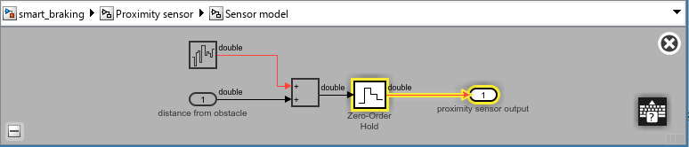
To find the source of the discretization, keep pressing the left arrow and note the colors of port names that reflect the sample time.

The Zero-Order Hold block in the Sensor model subsystem coverts the signal from continuous to discrete.