Temperature Measurement System Using Nonlinear Behavioral Data of Type S Thermocouple
This example shows how to build and simulate a temperature measurement system that uses a nonlinear dataset describing the behavior of a type S thermocouple.
In this example, the temperature measurement system consists of an Input Signal module and a Signal Processing module.
The
Input Signalmodule measures temperature using the nonlinear type S thermocouple model and generates an analog voltage signal from the temperature signal.The
Signal Processingmodule processes the analog voltage signal from theInput Signalmodule and maps the voltage values to temperature values using the nonlinear thermocouple data. The system displays these temperature values using a Scope block.
Open the model.
mdl = 'sldemo_tc.slx';
open_system(mdl)

Input Signal Module
The Input Signal module contains Thermocouple Model subsystem and a Unit Conversion block.
The Thermocouple Model contains a Transfer Fcn block and a Polynomial block.
open_system('sldemo_tc/Thermocouple Model')

The probe and bead dynamics of the type S thermocouple are modeled as a first-order system with time constant of 30 msec using the Transfer Fcn block. The nonlinear behavior of the system is modeled using the Polynomial block whose coefficients are obtained from NIST Standard Database 60 for a type S thermocouple from -50 to 1063 degC. For numerical stability, the coefficients are scaled to return voltage signal in microvolts unit.
Then, a Unit Conversion block converts the voltage signal in microVolt (mV) to a voltage signal in Volt(V). This analog voltage signal feeds into the Signal Processing module.
Signal Processing Module
The Signal Processing module contains two subsystems: AD Converter and Data Mapping.
AD Converter Subsystem
The AD Converter subsystem uses an anti-aliasing filter that pre-processes the analog voltage signal from the Input Signal module and feeds an Idealized ADC quantizer block. Then, the ADC quantizer converts the analog voltage signal to digital bits.
Open the AD Converter subsystem.
open_system('sldemo_tc/AD Converter');
Inside this subsystem, the pre-processing starts with adding a bias of 0.000236 to the analog voltage signal. Then, the signal is amplified to match the range of -0.235 mV to 18.661 mV (-50 degC to 1765 degC). To prevent aliasing, this signal is passed through a third-order Butterworth anti-aliasing filter designed for Wn of 15 Hz using the butter (Signal Processing Toolbox) function from the Signal Processing Toolbox™.
[num,den] = butter(3, 15*2*pi, 'low', 's')
The output of this anti-aliasing filter feeds a Sample and Hold block that drives the Idealized ADC quantizer block, which converts this analog signal voltage to digital bits. Since the sampling period is 20 msec, the conversion time is ignored as it is typically two orders of magnitude smaller for devices currently available. If the conversion time were an appreciable fraction of the sample period, it would not be ignored, as it would significantly affect system dynamics.
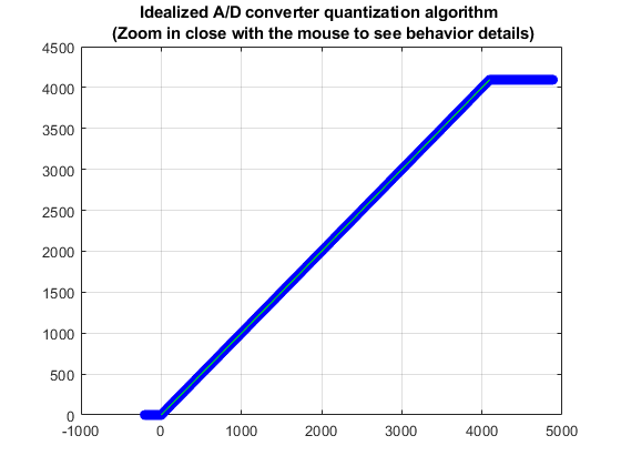
The quantization algorithm used by the Idealized ADC quantizer block takes in a 0 to 5 volt signal and outputs a 12-bit digital word in a 16-bit unsigned integer. A value of 0 corresponds to 0 V and a value of 4096 corresponds to 5 V. A change in the least significant bit (LSB) is about 1.2 mV. As 12 bits can only reach the value of 4095, the highest voltage that this device can read is approximately 4.9988 V. In order to have no more than 1/2 LSB error within the operating range, the quantizer changes values midway between each voltage point, resulting in a 1/2-width interval at 0 V and a 3/2-width interval just below 5 V. The last interval has one full LSB due to its 3/2-width size.
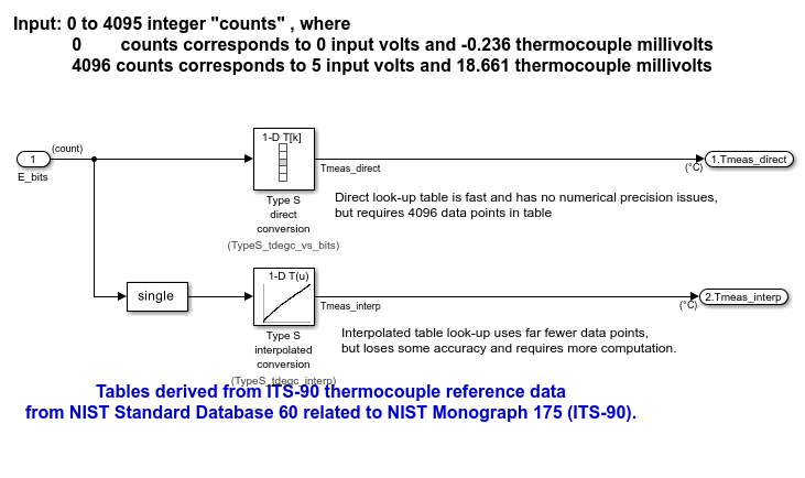
Data Mapping Subsystem
The Data Mapping subsystem maps the digital bits from the AD Converter subsystem to the temperature values using Lookup Table blocks, which use the nonlinear thermocouple data as table data and breakpoints. This subsystem receives a 16-bit unsigned integer from the ADC quantizer whose full scale range is 0 to 4095 counts, which corresponds to -0.235 mV and 18.6564 mV thermocouple loop voltage.
Open the Data Mapping subsystem.
open_system('sldemo_tc/Data Mapping')

Using the Standard Reference Database 60 from NIST Monograph 175, you can access the standard reference data that describes the behavior for the eight standard thermocouple types. This database relates thermocouple output to the International Temperature Scale of 1990. From this database, you have a complete set of temperature (T, degC) vs. voltage (E, mV) data, approximating polynomial coefficients, and inverse polynomial coefficients for the standard thermocouple types B, E, J, K, N, R, and S.
1-D Direct LUT - The Direct Lookup Table block uses table data that gives the thermocouple temperature that corresponds to each possible digital bit, which is an integer between 0 and 4095. The Table data variable
TypeS_tdegc_vs_bitsis defined in the model workspace. The Direct Lookup table block gives the best accuracy and performs the calculation faster than the 1-D Lookup Table block. However, because the 1-D Lookup Table block requires one number per ADC output value, and for a 12-bit ADC, it can be a burden in memory constrained environments. For double precision data, you need a 16 kB ROM.1-D LUT - The 1-D Lookup Table block uses both Table Data (bits) and its corresponding temperature (degC). This approach requires only 664 bytes of ROM. The Table data variable
TypeS_tdegc_interpand the Breakpoints 1 variableTypeS_bits_bpare defined in the model workspace. The 1-D Lookup Table block uses less ROM than the Direct Lookup Table block but it takes longer to compute than an indirect memory access. The 1-D Lookup Table block also introduces error into the measurement, which goes down as the number of points in the table increases.
Simulation and Results
Simulate the model. Observe that results from both 1-D Direct LUT and the 1-D LUT match and track the temperature signal received by the thermocouple. Direct look-up table is fast and has no numerical precision issues, but requires 4096 data points in table while the 1-D Lookup table uses far fewer data points, but loses some accuracy and requires more computation.
out = sim(mdl);
open_system('sldemo_tc/Scope')
References
[1] Burns, George W., Margaret G. Scroger, Gregory F. Strouse, Mary Carroll Croarkin, and William F. Guthrie. "Temperature-electromotive force reference functions and tables for the letter-designated thermocouple types based on the ITS-90." NASA STI/Recon Technical Report N 93 (1993): 3121. https://doi.org/10.6028/NIST.MONO.175
[2] Preston-Thomas, Hugh. "The International Temperature Scale of 1990(ITS-90)." metrologia 27, no. 1 (1990): 3-10.
[3] Kasap, Safa. "Thermoelectric effects in metals: thermocouples." Canada: Department of Electrical Engineering University of Saskatchewan (2001): 1-11.
See Also
Direct Lookup Table (n-D) | 1-D Lookup Table | Subsystem | Transfer Fcn | Polynomial