Build a Clutch Lockup Model

R2026b

This example shows how to model systems with discontinuous dynamics using Simulink® enabled subsystems by examining a clutch lockup model with switching friction modes. When modeling a clutch system, lockup introduces topological changes in system dynamics. When you model the clutch using enabled subsystems you can define separate dynamic models for different physical regimes that execute one at a time.

For an example of clutch dynamics in a conventional vehicle, see Build Conventional Vehicle Model (Powertrain Blockset) (Powertrain Blockset).

Clutch Dynamics and Mode Transitions

The clutch system in this example consists of two plates that transmit torque between the engine and transmission.

The system has two distinct modes of operation:

Slipping, when the two plates have differing angular velocities
Lockup, when the two plates rotate together

Handling the transition between these two modes presents a modeling challenge. When the system locks up, it loses a degree of freedom, and the transmitted torque exhibits a step discontinuity. The magnitude of the torque drops from the maximum value supported by the friction capacity to a value that is necessary to keep the two halves of the system spinning at the same rate. In the reverse transition, or break apart, the transmitted torque exceeds the friction capacity of the clutch plates.

Switching friction modes involves changing between sliding and sticking friction formulations as operating conditions change. This switch requires different equations and constraints to represent the system behavior accurately.

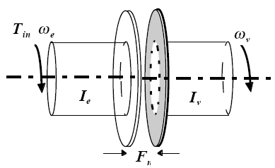
Clutch system showing engine inertia connected to vehicle inertia through friction plates. Engine torque drives rotation between the two sides.

System Variables

These are used in the analysis and modeling.

$T_{i n}$ = input (engine) torque

$F_{n}$ = normal force between friction plates

$I_{e}, I_{v}$ = moments of inertia for the engine and for the transmission/vehicle

$b_{e}, b_{v}$ = damping rates at the engine and transmission/vehicle sides of the clutch

$μ_{k}, μ_{s}$ = kinetic and static coefficients of friction

$ω_{e}, ω_{v}$ = angular speeds of the engine and transmission/vehicle input shafts

$r_{1}, r_{2}$ = inner and outer radii of the clutch plate friction surfaces

$R$ = equivalent net radius

$T_{c l}$ = torque transmitted through the clutch

$T_{l}$ = friction torque required of the clutch to maintain lockup

Equation Set 1

The state equations for the coupled system are derived as follows:

$I_{e} {ω_{}^{˙}}_{e} = T_{i n} - b_{e} ω_{e} - T_{c l}$

$I_{v} {ω_{}^{˙}}_{v} = T_{c l} - b_{v} ω_{v}$

Equation Set 2

The torque capacity of the clutch is a function of its size, friction characteristics, and the normal force that is applied.

$(T_{f})_{\max} = \int \int_{A} \frac{r \times F_{f}}{A} d a = \frac{F_{n} μ}{π (r_{2}^{2} - r_{1}^{2})} \int_{r_{1}}^{r_{2}} \int_{0}^{2 π} r^{2} d r d θ = \frac{2}{3} R F_{n} μ$

$R = \frac{r_{2}^{3} - r_{1}^{3}}{r_{2}^{2} - r_{1}^{2}}$

Equation Set 3

When the clutch is slipping, the model applies a friction torque equal to the maximum kinetic friction capacity, with its direction determined by the sign of the relative angular speed between the engine and vehicle so that the torque always opposes slip.

This equation gives the maximum torque magnitude the clutch can transmit while slipping:

$T_{f m a x k} = \frac{2}{3} R F_{n} μ_{k}$

This equation applies a direction to the torque calculated previously:

$T_{c l} = s gn (ω_{e} - ω_{v}) T_{f m a x k}$

where sgn denotes the sign function.

Equation Set 4

When the clutch is locked, the angular velocities of the engine and transmission input shafts are the same. The system torque then acts on the combined inertia as a single unit. The differential equations from Equation Set 1 are combined into a single equation for the locked state.

$ω_{e} = ω_{v} = ω$

$(I_{e} + I_{v}) ω_{}^{˙} = T_{i n} - (b_{e} + b_{v}) ω$

Equation Set 5

Solving Equation Set 1 and Equation Set 4, the torque transmitted by the clutch while locked is:

$T_{c l} = T_{f} = \frac{I_{v} T_{i n} - (I_{v} b_{e} - I_{e} b_{v}) ω}{I_{v} + I_{e}}$

Equation Set 6

The clutch thus remains locked unless the magnitude of $T_{f}$ exceeds the static friction capacity, $T_{f m a x s}$ .

$T_{f m a x s} = \frac{2}{3} R F_{n} μ_{s}$

This state diagram describes the overall behavior of the clutch.

Opening the Model and Running the Simulation

Open the model. The model uses two enabled subsystems: the Locked subsystem and the Unlocked subsystem. The simulation can use one subsystem while the clutch is slipping and the other when the clutch is locked. This configuration enables the initialized states of one subsystem to match the state values immediately prior to the switch.

Run the model using the default inputs to observe transitions between slipping and locked clutch operation.

The model logs relevant data to MATLAB® workspace in a structure called sldemo_clutch_output. For information about signal logging, see Mark Signals for Logging.

open_system('sldemo_clutch');
evalc('sim(''sldemo_clutch'')');

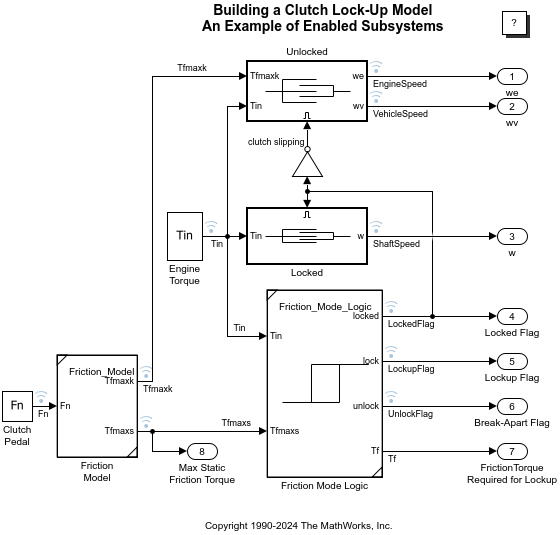
Clutch lockup model with unlocked and locked enabled subsystems and friction mode logic controlling state transitions.

Modeling Slip Dynamics in an Enabled Subsystem

Double-click the Unlocked subsystem in the model window canvas to view the subsystem contents. This subsystem models both sides of the clutch, coupled by the friction torque. It is constructed around the Integrator blocks, which calculate engine and vehicle speeds. The model uses Gain, Product, and Sum blocks to compute the speed derivatives (acceleration) from the states and the subsystem inputs of engine torque, Tin, and clutch capacity, Tfmaxk.

open_system('sldemo_clutch/Unlocked');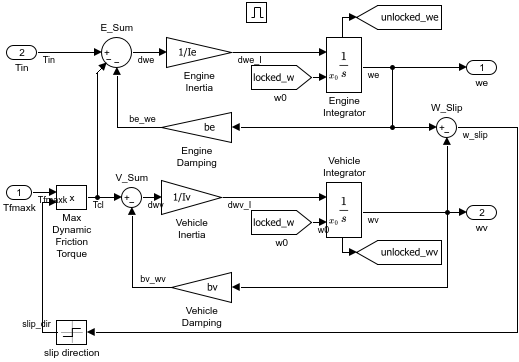

Unlocked enabled subsystem modeling slip dynamics. Engine and vehicle integrators compute angular velocities from torque inputs, inertia, and damping, and the subsystem is enabled during slipping.

The Enable block at the top of the diagram defines the model as an enabled subsystem:

An enable input appears on the subsystem block, identified by the pulse-shaped symbol used on the Enable block itself.
The subsystem executes only when the signal at the enable input is greater than zero.

In this example, the Unlocked subsystem executes only when the supervising system logic determines that it should be enabled.

When the system is enabled, the simulation must reinitialize the integrators to begin simulating from the correct point. In this case, both sides of the clutch are moving at the same velocity the moment the clutch unlocks. The Unlocked subsystem, which had been inactive, needs to initialize both integrators at that speed in order to keep the system speeds continuous.

The simulation uses From blocks to communicate the state of the locked speed to the initial condition inputs of the two integrators. Each From block represents an invisible connection between itself and a Goto block somewhere else in the system. The Goto blocks connect to the state ports of the integrators so that the model can use these states elsewhere in the system without explicitly drawing in the connecting lines.

Modeling Locked-State Dynamics with State Handoff

The Locked subsystem is another enabled subsystem in the clutch model. This subsystem uses a single state to represent the engine and vehicle speeds. It computes acceleration as a function of the speed and input torque. As in the Unlocked subsystem, a From block provides the integrator initial conditions and a Goto block broadcasts the state for use elsewhere in the model. While simulating, either the Locked or the Unlocked subsystem is active at all times. Whenever the control changes, the states are handed off between the two subsystems.

open_system('sldemo_clutch/Locked');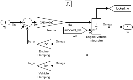

Locked enabled subsystem modeling lockup dynamics. A single integrator computes shared angular velocity from torque input and combined damping.

Detecting and Managing Friction Mode Transitions

The Friction Mode Logic subsystem computes the static and kinetic friction (with the appropriate friction coefficient) according to this formula:

$T_{f m a x} = \frac{2}{3} R F_{n} μ$

The Lockup Detection Subsystem block uses velocity-match detection with a Hit Crossing block and checks if required friction torque is less than or equal to Tfmaxs to issue a lock request.

The Break Apart Detection Subsystem block issues an unlock command when actual friction torque is greater than or equal to Tfmaxs.

Open the Friction Mode Logic subsystem by double-clicking it. You can also right-click and select System Mask > Look Inside Mask.

open_system('Friction_Mode_Logic');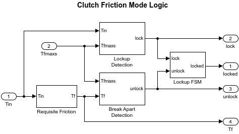

Friction Mode Logic subsystem with detection logic, a Lockup FSM for state output, and a block computing friction torque.

Other Components

The other blocks in the system calculate the torque required for lockup, Equation Set 5, and implement the logic described in the state diagram. In the Lockup Detection subsystem within the Friction Mode Logic subsystem, the Hit Crossing block named Velocities Match precisely locates the instant at which the clutch slip reaches zero. This action allows the mode to transition at the right moment.

System Inputs

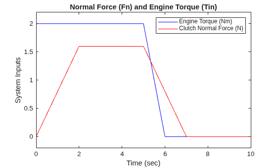
The system inputs are normal force, Fn, and engine torque, Tin. Each input is represented by a matrix table in the model workspace. You can visualize various signals by selecting the corresponding boxes on the Clutch Demo Signals dialog box.

plot(sldemo_clutch_output.get('Tin').Values.Time, ...
     sldemo_clutch_output.get('Tin').Values.Data, 'b', ...
     sldemo_clutch_output.get('Fn').Values.Time,  ...
     sldemo_clutch_output.get('Fn').Values.Data,  'r'  );
xlabel('Time (sec)');
ylabel('System Inputs');
legend('Engine Torque (Nm)', 'Clutch Normal Force (N)');
title('Normal Force (Fn) and Engine Torque (Tin)');
axis([0 10 -.2 2.2]);

Figure contains an axes object. The axes object with title Normal Force (Fn) and Engine Torque (Tin), xlabel Time (sec), ylabel System Inputs contains 2 objects of type line. These objects represent Engine Torque (Nm), Clutch Normal Force (N).

Interpreting Simulation Results Across Lockup Events

These parameter values are used in the simulation. These values are not meant to represent the physical quantities corresponding to an actual system, but rather to facilitate a baseline example.

$I_{e} = 1 k g \cdot m^{2}$
$I_{v} = 5 k g \cdot m^{2}$
$b_{e} = 2 N m / r a d / s e c$
$b_{v} = 1 N m / r a d / s e c$
$μ_{k} = 1$
$μ_{s} = 1.5$
$R = 1 m$

For these inputs, the system velocities behave as shown in this figure. The simulation begins in the unlocked mode, producing an initial engine speed flare as the engine accelerates relative to the larger vehicle-side inertia. At about $t = 4 s e c$ , the velocities come together and remain locked, indicating that the clutch capacity is sufficient to transmit the torque. After $t = 5 s e c$ , the engine torque begins to decrease, as does the normal force on the friction plates. Consequently, the onset of slip occurs at about $t = 6.25 s e c$ as indicated by the separation of the engine and vehicle speeds.

plot(sldemo_clutch_output.get('EngineSpeed').Values.Time, ...
     sldemo_clutch_output.get('EngineSpeed').Values.Data,  'r', ...
     sldemo_clutch_output.get('VehicleSpeed').Values.Time, ...
     sldemo_clutch_output.get('VehicleSpeed').Values.Data, 'b', ...
     sldemo_clutch_output.get('ShaftSpeed').Values.Time, ...
     sldemo_clutch_output.get('ShaftSpeed').Values.Data,   'g'  );
xlabel('Time (sec)');
ylabel('Angular Speed (rad/sec)');
legend('\omega_e - Engine Speed', '\omega_v - Vehicle Speed', '\omega - Shaft Speed');
title('Angular Velocities for Default Inputs');

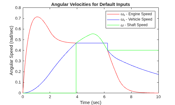
$Figure contains an axes object. The axes object with title Angular Velocities for Default Inputs, xlabel Time (sec), ylabel Angular Speed (rad/sec) contains 3 objects of type line. These objects represent \omega_e - Engine Speed, \omega_v - Vehicle Speed, \omega - Shaft Speed.$

The various states remain constant while they are disabled. At the time instants at which transitions take place, the state hand-off is both continuous and smooth. When a state is enabled, each integrator is supplied with the appropriate initial conditions to use.

These results show how enabled subsystems and explicit state handoff maintain continuity during dynamic mode switching. The sharp yet well-resolved transitions demonstrate how hit-crossing detection enables accurate simulation of discontinuities.

close_system('sldemo_clutch',0);
clear sldemo_clutch_output;