Exploring the Solver Jacobian Structure of a Model
The example shows how to use Simulink® to explore the solver Jacobian sparsity pattern, and the connection between the solver Jacobian sparsity pattern and the dependency between components of a physical system. A Simulink model that models the synchronization of three metronomes placed on a free moving base are used.
The Solver Jacobian Pattern
In general, the continuous part of a Simulink model can be written as:

where  are the continuous states and
  are the inputs.
  are the outputs.
The matrix:

is called the system solver Jacobian matrix. When an implicit ODE solver is used to solve the system equations,  needs to be computed when needed. For example, the Jacobian matrix of a set of first order ODEs

is
![$$ J_x = \left[ {\begin{array}{*{20}c} {\frac{{\partial f_1 }}{{\partial x_1 }}} & {\frac{{\partial f_1 }}{{\partial x_2 }}} \\ {\frac{{\partial f_2 }}{{\partial x_1 }}} & {\frac{{\partial f_2 }}{{\partial x_2 }}} \\ \end{array}} \right] = \left[ {\begin{array}{*{20}c} {x_2 } & {x_1 } \\ 0 & 1 \\ \end{array}} \right] $$](../../examples/simulink_general/win64/sldemo_metroExample_eq11832656377446100082.png)
You can convert the solver Jacobian matrix to a Boolean sparse matrix by representing each non-zero element as 1, and each element that is always zero (hard zero) as 0. For example, the Boolean matrix corresponding to above Jacobian is:
![$$ J_{xp} = \left[ {\begin{array}{*{20}c} 1 & 1 \\ 0 & 1 \\ \end{array}} \right], $$](../../examples/simulink_general/win64/sldemo_metroExample_eq04339857009896876157.png)
where  is called the solver Jacobian pattern matrix.
The solver Jacobian pattern matrix can be generated directly from the original system equations by using the following rule:
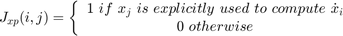
As you can see, the solver Jacobian pattern matrix actually represents the dependency between the state variables and their derivatives. If computing of  needs the value of
  , then there exists a dependency
  and
and  . These dependencies are determined by the physical nature of the system, and thus by studying the solver Jacobian matrix, you can explore the physical structure of the physical system represented by the model. Simulink provides APIs for the user to get the solver Jacobian pattern matrix. The following shows how to access the solver Jacobian pattern and to use it to the study the model.
The Pattern and Dependency: Synchronization of Metronomes
Synchronization is defined as an adjustment of rhythms of oscillating objects due to their weak interaction [1]. One of the first scientifically documented observations of synchronization was reported by the Dutch scientist Christiaan Huygens, the inventor of pendulum clock [2]. Huygens discovered that two pendulums attached to the same beam supported by chairs would swing in exact opposite direction after some time. A similar set up used in this example is shown in Figure 1.
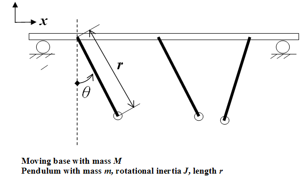
Figure 1: Set up used in this example: three metronomes on a moving base
Modeling the System
The model of this physical system can be divided into two parts:
The metronomes mechanism
The moving base
The metronomes mechanism
Referring to Figure 1, the dynamic equations of a single metronome on a moving base can be derived as[3]:
![$$ \underbrace {\ddot \theta }_{Angular~acceleration} + \underbrace {\frac{{mrg}}{J}\sin \theta }_{Gravitational~term} + \underbrace {\frac{b}{J}\left[ {\left( {\frac{\theta }{{\theta _r }}} \right)^2 - 1} \right]\dot \theta }_{Escapement~and~damping~term} + \underbrace {\left( {\frac{{rm\cos \theta }}{J}} \right)\ddot x}_{Coupled~inertial~force~term} = 0~~~~~~~~~~(eq.1) $$](../../examples/simulink_general/win64/sldemo_metroExample_eq05664120881427947847.png)
The first two terms describe a simple pendulum without friction. The third term is used to approximate the escapement* and any damping of the metronome. This term increases the angular velocity for  and decreases it for
  [3]. The last term is the coupled effect from the moving base, in terms of an inertial force.
The moving base
Assuming the motion of the base is frictionless, then the center of mass of the system will not change and you can be derive the following:
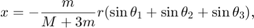
where  is the mass of the base and
  is the mass of the pendulum.
Then eq.1 can be changed to:
![$$ \ddot x = - \frac{m}{{M + 3m}}r\left[ {\ddot \theta _1 \cos \theta _1 - \sin \theta _1 (\dot \theta _1 )^2 + \ddot \theta _2 \cos \theta _2 - \sin \theta _2 (\dot \theta _2 )^2 + \ddot \theta _3 \cos \theta _3 - \sin \theta _3 (\dot \theta _3 )^2 } \right]~~~~~~~~~~(eq.2) $$](../../examples/simulink_general/win64/sldemo_metroExample_eq02469793368176530282.png)
The following shows the above system implemented using Simulink. The model contains three metronome subsystems and the moving base.
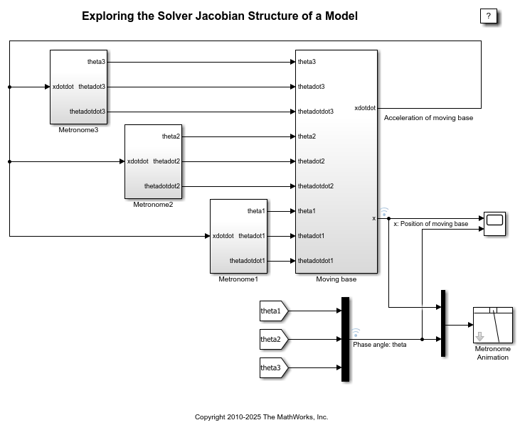
Figure 2: The Simulink model of the metronomes system
Simulation of this system shows an interesting phenomenon: Synchronization. It shows that all three metronomes with different initial phase angle eventually become synchronized with each other. Figure 3 shows the simulation results. The main cause for synchronization is the moving base that links all these metronomes together. This physical connection can be observed from the dynamic equation of each metronome.
Also, this physical connection can also be observed from the solver Jacobian pattern of this model. The following MATLAB® code shows how to get the solver Jacobian pattern.
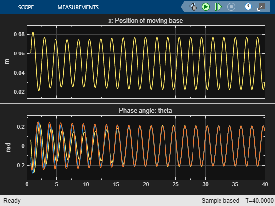
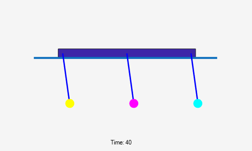
Figure 3: The synchronized metronomes
Steps to Get the Solver Jacobian Pattern
% 1. Set the solver to be any implicit solver
set_param(mdl, 'Solver', 'ode15s');
% 2. Set the solver Jacobian method to be Sparse perturbation *
set_param(mdl, 'SolverJacobianMethodControl', 'SparsePerturbation');
% 3. Get the solver Jacobian object.
   J = Simulink.Solver.getSlvrJacobianPattern(mdl);
   disp('J = ');
   disp(J);
% 4. Show the pattern in a figure. use the method J.show
J.show;
% 5. Explore the pattern with the given state name and other information
   stateNames = J.stateNames;
   disp('stateNames = ');
   disp(stateNames);
The results you will see are:
J =
  SlvrJacobianPattern with properties:

        Jpattern: [8×8 double]
     numColGroup: 6
        colGroup: [8×1 double]
      stateNames: {8×1 cell}
    blockHandles: [8×1 double]

stateNames =
    {'sldemo_metro/Moving base/Integrator1'              }
    {'(sldemo_metro/Metronome1/Integrator2).(Theta1)'    }
    {'(sldemo_metro/Metronome2/Integrator2).(Theta2)'    }
    {'(sldemo_metro/Metronome3/Integrator2).(Theta3)'    }
    {'(sldemo_metro/Metronome3/Integrator1).(Thetadot_3)'}
    {'(sldemo_metro/Metronome2/Integrator1).(Thetadot_2)'}
    {'(sldemo_metro/Metronome1/Integrator1).(Thetadot_1)'}
    {'sldemo_metro/Moving base/Integrator'               }
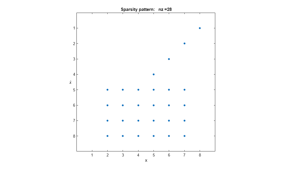
Figure 4: The solver Jacobian pattern
Properties of the Solver Jacobian Pattern Object
The solver Jacobian pattern J is an object. It contains the following properties:
Jpattern: A sparse mxArray which is the Jacobian pattern.
numColGroup: Number of column groups.
colgroup: A column partition of the sparse pattern matrix.
stateNames: A cell array containing the state name of each state.
blockHandles: Block handles of the owner of each state.
Study of the Solver Jacobian Pattern
Referring to Figure 4. First, the solver Jacobian of this model is sparse and the number of non-zero element is 28. Secondly, the number of column groups is 6; is less than the number of states 8.
The row 1-4 indicates the following dependencies:
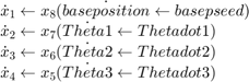
These relations are clear since speed is the derivative of position. Row 5-8 shows the following relations:

These relations show that to compute the angular acceleration of the metronomes or acceleration of the moving base, the angular position and angular speed of the metronomes are needed, but not the position and speed of the base. These relations can be found by studying eq.(1) and eq.(2) directly.
Conclusion
The Solver Jacobian pattern is a tool to study the data dependency relations between the derivatives of the state variables and the state variables. These relations usually reflect certain physical couplings in the physical system. By using the tools provided, you can discover these relations associated with a Simulink model, even without the original dynamic equations of the physical model.
References
[1] Arkady Pikosvky, Michael Rosenblum, and Jurgen Kurths. Synchronization. Cambridge University Press, 2001.
[2] Ward T. Oud, Design and experimental results of synchronizing metronomes, inspired by Christiaan Huygens, Master Thesis, Eindhoven University of Technology, 2006.
[3] Pantaleone, James, American Journal of Physics, Volume 70, Issue 10, pp. 992-1000, 2002.
Escapement is a set of mechanism that drives the metronome. See [2] for more details.