Explore Variable-Step Solvers with Stiff Model
This example shows the behavior of variable-step solvers in a Foucault pendulum model. Simulink® solvers ode45, ode15s, ode23, and ode23t are used as test cases. Stiff differential equations are used to solve this problem. There is no exact definition of stiffness for equations. Some numerical methods are unstable when used to solve stiff equations and very small step sizes are required to obtain a numerically stable solution to a stiff problem. A stiff problem may have a fast changing component and a slow changing component.
Foucault pendulum is an example of a stiff problem. The pendulum completes an oscillation in a few seconds (fast changing component) whereas the Earth completes a rotation about its axis in a day (slow changing component). The oscillation plane of the pendulum slowly rotates because of Earth's axial rotation. You can read more about the physics of a Foucault pendulum in Modeling a Foucault Pendulum.
The simulation calculates the position of the pendulum bob in the x-y plane as viewed by an observer on the surface of Earth. The total energy of the pendulum is then calculated and used to assess the performance of various Simulink solvers.
Foucault Pendulum Model
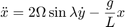
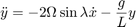
The Foucault pendulum is described by the system of coupled differential equations shown below. Friction and air drag are not taken into consideration (this greatly simplifies the equations). A full derivation of these equations is given in the Foucault Pendulum example.


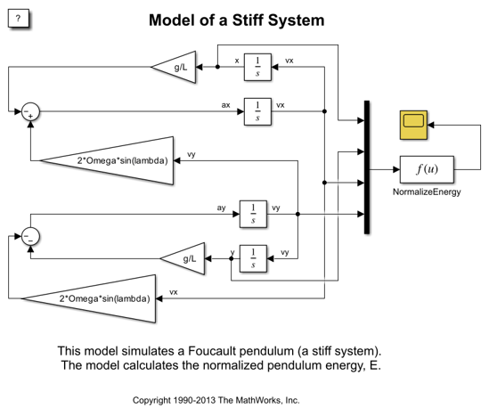
The model sldemo_solvers is used to solve the differential equations that describe a Foucault pendulum. The example simulates a Foucault pendulum for 86,400 seconds. The constants and initial conditions are saved the model workspace.
Variable-Step Solvers
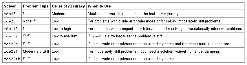
This example investigates the performance of the ode45, ode15s, ode23, and ode23t variable-step solvers.
Assessing Solver Performance
There are different ways to assess the performance of a solver. If a problem has a closed form solution, you could compare the solver results with the expected theoretical result. You could also monitor the time it takes to simulate a model using a particular solver.
Unfortunately there is no exact theoretical solution for the Foucault Pendulum problem. There is an approximate closed form solution. However you cannot use the approximate closed form solution to assess solver performance (see the Foucault pendulum example).
Total Energy Conservation
This example assesses solver performance by verifying the energy conservation law. In a frictionless environment, the total energy of the pendulum must remain constant. The calculated energy of the pendulum, however, does not remain constant as a result of limited numeric accuracy.
This example calculates the normalized total energy of the pendulum at every time step. The relative error in energy equals the change in total energy over the course of the simulation. Ideally, the relative error in energy must be zero because energy is conserved. Total energy is the sum of potential and kinetic energy. The NormalizeEnergy block calculates the normalized pendulum energy using these equations:

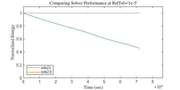
The plot shows the normalized energy versus time as calculated using ode23 and ode23t. In this particular problem ode23t is much more accurate than ode23. In the simulation that used ode23, the normalized pendulum energy decreased by more than 60%. A pendulum with lower energy has a lower oscillation amplitude. You can see this effect in the next plot, where the amplitude of the pendulum calculated by ode23 decreases as the oscillation plane rotates.
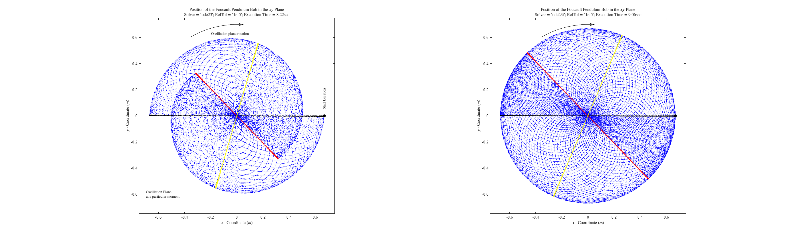
These plots illustrate the difference between a stiff and a non-stiff solver. Each plot shows the position of the pendulum bob throughout a day. Every 15th data point is plotted as a blue point. The black dot marks the initial position of the pendulum bob and the black line marks the initial pendulum oscillation plane. The red line indicates the oscillation plane after a day. The yellow line shows the oscillation plane at some intermediate point in time. The oscillation plane of the pendulum does not complete a full rotation within a day. How fast the oscillation plane rotates depends on the geographical latitude (see details in the Foucault pendulum example). The pendulum amplitude in the left plot decreases whereas the amplitude in the right plot remains constant. For the same relative tolerance of 1e-5, the stiff solver gives a more accurate result but requires more execution time.
The next plots show a more detailed performance study of Simulink solvers. Four solvers were chosen to illustrate how relative error and execution time vary as a function of relative tolerance. You can use the script sldemo_solvers_mcode.m for more extensive solver tests. This script generates C code from the model to speed up the simulations and can take several minutes to run.
Building RSim executable for model..
Time taken: 60.514479 seconds.

Running generated RSim executable..
Time taken: 82.698950 seconds.

In this example, the relative error does not decrease significantly for relative tolerance values smaller than 1e-6. This is a numeric solver limitation that depends on the particular model. Reducing the solver relative tolerance does not necessarily improve accuracy. You need to estimate the minimal accuracy that is required for your problem and choose the solver accordingly to balance simulation costs. For example, you might want to know the position of the Foucault pendulum bob within a few centimeters. Calculating the position of a pendulum within a few microns is not necessary because you cannot measure the position that accurately.
The numeric results and behavior of a simulation can differ depending on solver settings. This is crucial in the case of stiff problems. When working with stiff models, choose a solver that will give an accurate result with lower computational cost. The relative tolerance for a variable-step solver or the step size for a fixed-step solver has to be small enough that the result is numerically stable. Although some solvers are more efficient than others, stiff solvers are better suited for solving stiff problems. Variable-step solvers are more robust than fixed-step solvers.