Spectrum Analyzer

R2026b

Display frequency spectrum

Libraries:
DSP System Toolbox / Sinks
Audio Toolbox / Sinks
DSP System Toolbox HDL Support / Sinks

Description

The Spectrum Analyzer block, referred to here as the scope, displays frequency-domain signals and the frequency spectrum of time-domain signals. The scope shows the spectrum view and the spectrogram view. The block algorithm performs spectral estimation using the filter bank method and Welch's method of averaged modified periodograms. You can customize the spectrum analyzer display to show the data and the measurement information that you need. For more details, see Algorithms.

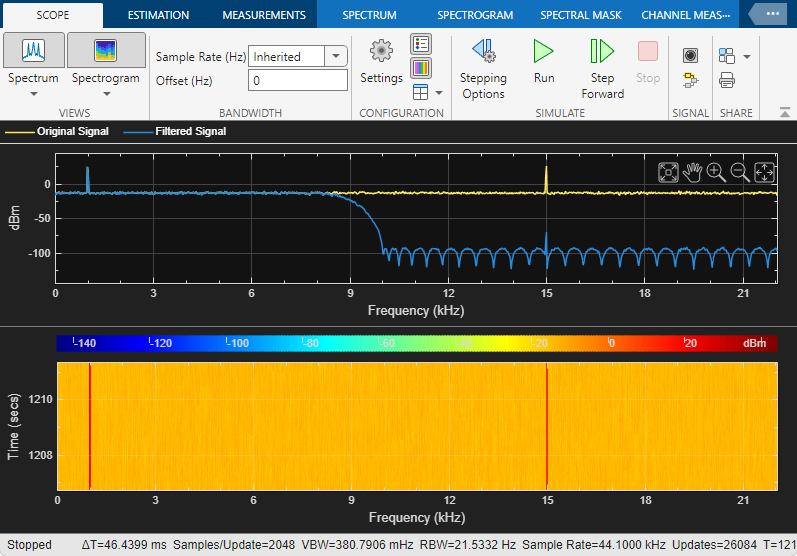
Snapshot of spectrum analyzer scope showing both the spectrum and the Spectrogram.

You can use the Spectrum Analyzer block in models running in Normal or Accelerator simulation modes. You can also use the Spectrum Analyzer block in models running in Rapid Accelerator or External simulation modes with some limitations.

You can use the Spectrum Analyzer block inside all subsystems and conditional subsystems. Conditional subsystems include enabled subsystems, triggered subsystems, enabled and triggered subsystems, and function-call subsystems. See Conditionally Executed Subsystems Overview for more information.

Measurements

Cursor Measurements — Measure signal values using vertical cursors.
Peak Finder Measurements — Find maxima and show the x-axis values at which they occur.
Channel Measurements — Measure the occupied bandwidth or adjacent channel power ratio (ACPR).
Distortion Measurements — Measure harmonic distortion and intermodulation distortion.
Spectral Mask — Visualize spectrum limits and compare spectrum values to specification values.

Programmatic Control

Configure and display the spectrum analyzer settings from the command line with the SpectrumAnalyzerBlockConfiguration (DSP System Toolbox) object.

Examples

expand all

Display Frequency Input on Spectrum Analyzer

This example uses:

Open Model

This example shows how to visualize frequency input signals with the Spectrum Analyzer block.

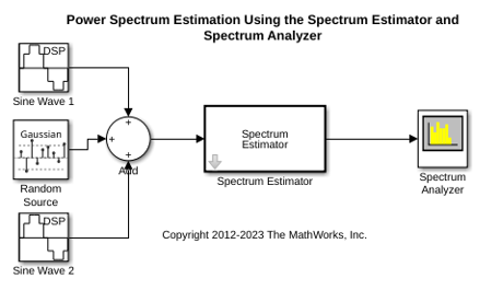
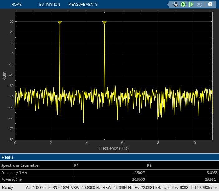
To visualize frequency-domain input signals using a Spectrum Analyzer block, set Input Domain to Frequency in the Home tab of the spectrum analyzer toolstrip. Click the Frequency Span drop-down arrow and clear the Two-Sided Spectrum parameter.

Run the model. You can see two peaks. To measure the peaks, enable Peak Finder in the Measurements tab.

Display Variable-Size Input Signals on Spectrum Analyzer

This example uses:

Open Model

Decimate a sinusoidal signal by varying the decimation factor using the Variable FIR Decimation (DSP System Toolbox) block. You can vary the decimation factor in the block dialog box or through an input port while the simulation is running.

Open and Inspect Model

Open the DisplayVariableSizeSignalonSpectrumAnalyzer model.

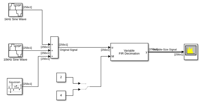
The input signal in the model is a sum of two sine waves with the frequencies of 1 kHz and 10 kHz, sample time of 1/44100 s, and contains 256 samples per frame. The Random Source block adds zero-mean white Gaussian noise with a variance of 0.05 to the sum of sine waves.

Pass this signal through the Variable FIR Decimation block. The Maximum decimation factor parameter in the block is set to 24. You can specify the decimation factor through the input port and vary it using the Manual Switch block. The output of the Variable FIR Decimation block is a variable-size signal whose frame size varies according to the decimation factor that you specify.

Run Model

Visualize the spectrum of the decimated signal in the spectrum analyzer. The sample rate of the spectrum analyzer updates based on the frame size of the signal and the sample rate of the signal.

When you set the decimation factor to 2, the output frame size is half the input frame size, and the spectrum analyzer uses a sample rate of 44100/2 or 22.05 kHz.

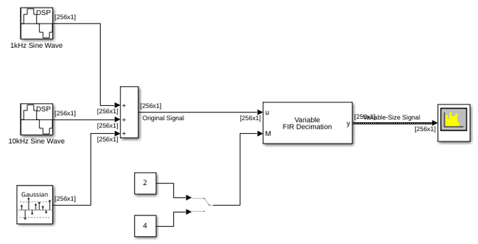
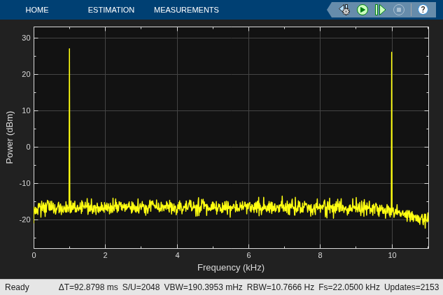
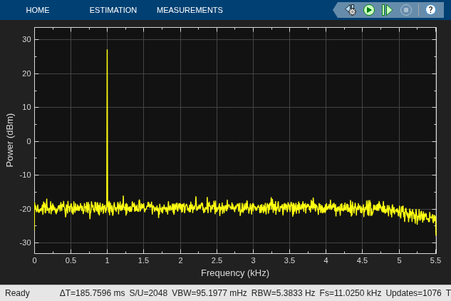
While the simulation is running, change the decimation factor to 4. You can see that the sample rate of the spectrum analyzer adjusts to 44100/4 or 11.025 kHz. The tone at 1 kHz remains the same while the tone at 10 kHz is no longer visible in the spectrum analyzer since the span of the spectrum is now [0 Fs/2] = [0 5.5125 kHz].

Obtain Measurements Data Programmatically for Spectrum Analyzer Block

This example uses:

Open Model

Compute and display the power spectrum of a noisy sinusoidal input signal using the Spectrum Analyzer block. Measure the cursor placements, adjacent channel power ratio, distortion, and peak values in the spectrum by enabling these block configuration properties:

CursorMeasurements
ChannelMeasurements
DistortionMeasurements
PeakFinder

Open and Inspect the Model

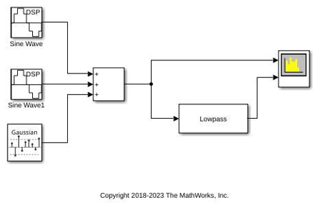
Filter a streaming noisy sinusoidal input signal using a Lowpass Filter block. The input signal consists of two sinusoidal tones: 1 kHz and 15 kHz. The noise is white Gaussian noise with a mean of 0 and a variance of 0.05. The sampling frequency is 44.1 kHz. Open the model and inspect the parameter values in the blocks.

model = 'spectrumanalyzer_measurements.slx';
open_system(model)

Access the configuration properties of the Spectrum Analyzer block using the get_param function.

sablock = 'spectrumanalyzer_measurements/Spectrum Analyzer';
cfg = get_param(sablock,'ScopeConfiguration');

Enable Measurements Data

To obtain the measurements, set the Enabled property to true. Label the peak measurements.

cfg.CursorMeasurements.Enabled = true;
cfg.ChannelMeasurements.Enabled = true;
cfg.DistortionMeasurements.Enabled = true;
cfg.PeakFinder.Enabled = true;
cfg.PeakFinder.LabelPeaks = true;

Simulate the Model

Run the model. The Spectrum Analyzer block compares the original spectrum with the filtered spectrum.

sim(model)

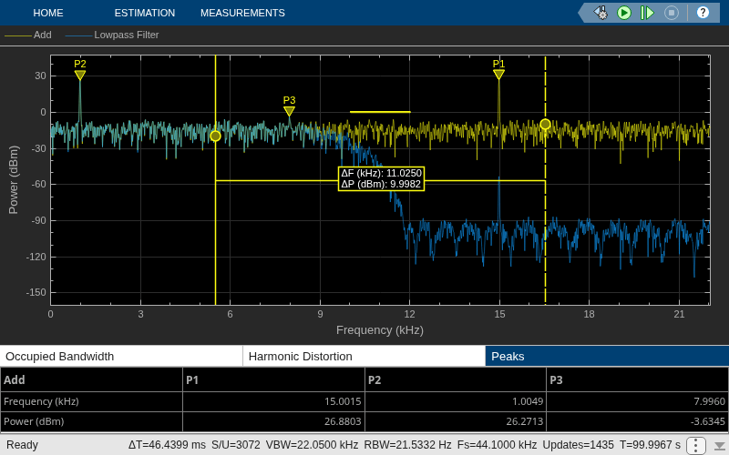
The panels at the bottom of the spectrum analyzer window display the measurements that you have enabled.

Use getMeasurementsData function

Use the getMeasurementsData function to obtain the measurements programmatically.

data = getMeasurementsData(cfg)

data =

  1×5 table

    SimulationTime    PeakFinder    CursorMeasurements    ChannelMeasurements    DistortionMeasurements
    ______________    __________    __________________    ___________________    ______________________

     {[99.9967]}      1×1 struct        1×1 struct            1×1 struct               1×1 struct

The values shown in the measurement panels match the values shown in data. You can access the individual fields of data to obtain the various measurements programmatically.

Compare Peak Values

As an example, compare the peak values. Verify that the peak values obtained by data.PeakFinder match with the values in the spectrum analyzer window.

peakvalues = data.PeakFinder.Value
frequencieskHz = data.PeakFinder.Frequency/1000

peakvalues =

   26.8803
   26.2713
   -3.6345


frequencieskHz =

   15.0015
    1.0049
    7.9960

Extended Examples

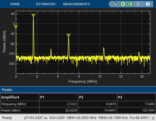
Spectrum Analyzer Measurements

Use the Spectrum Analyzer block for harmonic distortion measurements (such as THD, SNR, SINAD, and SFDR), third-order intermodulation (TOI) distortion measurements, and adjacent channel power ratio (ACPR) measurements. The example also shows you how to view time-varying spectra by using a spectrogram and automatic peak detection. The example includes five amplifier models, with each model representing a typical setup to perform one of the measurements.

(DSP System Toolbox)

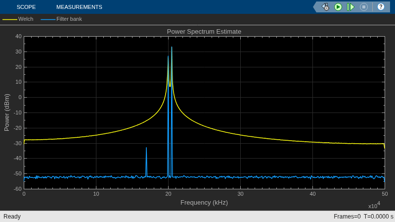
High Resolution Spectral Analysis in Simulink

Perform spectral estimation in Simulink^® using the filter bank method, and compare the performance with the Welch's averaged modified periodogram method.

(DSP System Toolbox)

Ports

Input

expand all

u — Signals to visualize
scalar | vector | matrix | array

Connect the signals you want to visualize. You can have up to 96 input ports. Input signals must have these characteristics:

Signal Domain — Frequency or time signals.
Type — Discrete signals.
Data type — Any data type that Simulink supports. See Data Types Supported by Simulink.
Dimension — One dimensional (vector), two dimensional (matrix), or multidimensional (array) signals. Input signal must have a fixed number of channels. See Signal Dimensions and Determine Signal Dimensions.

The Spectrum Analyzer block supports variable-size input signals, that is, the frame size of the signals can change during simulation. When the signal frame size changes, the sample rate the scope uses changes accordingly, which in turn updates the frequency span of the spectrum display.

The Spectrum Analyzer block accepts fixed-point input, but converts it to double for display.

This port is unnamed until you enable one of these inputs ports:

F
RBW
VBW

(since R2024a)

F — Frequencies in Hz
column vector

Specify the frequencies in Hz. The frequency vector must be a finite, monotonically increasing, column vector with two or more elements. The number of frequency vector points must be equal to the input frame size. You can also specify the frequencies using the Frequency Vector (Hz) parameter on the Home tab under the Frequency Span drop-down.

Dependencies

To enable this port, on the Home tab:

Set Input Domain to Frequency.
Click the Frequency Span drop-down arrow and set Frequency Vector to Input Frequency Vector.

RBW — RBW Value
positive scalar

Specify the resolution bandwidth in Hz through this port. RBW defines the smallest positive frequency that can be resolved by the scope. You can also specify the RBW value using the RBW (Hz) parameter on the Estimation tab.

Dependencies

To enable this port, set RBW (Hz) to Input port on the Estimation tab.

VBW — VBW Value
positive scalar

Specify the video bandwidth in Hz through this port. Video bandwidth is the bandwidth of the lowpass filter that the scope uses to average or smooth the noise in the signal before displaying it. You can also specify the VBW value using the VBW (Hz) parameter on the Estimation tab.

Dependencies

To enable this port, set:

Input Domain to Time on the Home tab.
Averaging Method to VBW on the Estimation tab.
VBW (Hz) to Input port on the Estimation tab.

Parameters

expand all

Home Tab

Views

Spectrum — Enable spectrum display
button

Select Spectrum to enable the spectrum display. Click the Spectrum drop-down arrow and select one of these signal traces.

Normal Trace — Plot the power spectral estimate.
Max-Hold Trace — Plot the running maximum of the power spectral estimate.
Min-Hold Trace — Plot the running minimum of the power spectral estimate.

Trace Settings

Normal Trace — Plot power spectral estimate
`on` (default) | `off`

When you select this check box, the spectrum analyzer calculates and plots the power spectral estimates. The spectrum analyzer performs a smoothing operation by averaging several spectral estimates and continues its spectral computations even when you clear this parameter.

Tunable: Yes

Dependencies

To clear this check box, first select Max-Hold Trace or Min-Hold Trace.

To show the normal trace in the scope display, select Spectrum on the Home tab.

Programmatic Use

Block Parameter: PlotNormalTrace

Type: logical

Max-Hold Trace — Plot running maximum of power spectral estimate
`off` (default) | `on`

Select this check box to plot the running maximum of the power spectral estimate. The spectrum analyzer computes the maximum-hold spectrum at each frequency bin by keeping the maximum value of all the power spectrum estimates. When you clear this check box, the spectrum analyzer resets its maximum-hold computations.

Tunable: Yes

Dependencies

To show the max-hold trace, select Spectrum on the Home tab.

Programmatic Use

Block Parameter: PlotMaxHoldTrace

Type: logical

Min-Hold Trace — Plot running minimum of power spectral estimate
`off` (default) | `on`

Select this check box to plot the running minimum of the power spectral estimate. The spectrum analyzer computes the minimum-hold spectrum at each frequency bin by keeping the minimum value of all the power spectrum estimates. When you clear this check box, the spectrum analyzer resets its minimum-hold computations.

Tunable: Yes

Dependencies

To show the min-hold trace, select Spectrum on the Home tab.

Programmatic Use

Block Parameter: PlotMinHoldTrace

Type: logical

Tunable: Yes

Spectrogram — Enable spectrogram display
button

Select Spectrogram to enable the spectrogram display. Click the Spectrogram drop-down arrow to customize the time span, time resolution, and the time orientation (vertical or horizontal).

Channel and Time Settings

Spectrogram Channel — Channel for which spectrogram is plotted
`1` (default) | character vector of a positive integer | string scalar of a positive integer

Select the signal channel for which the spectrogram settings apply.

Tunable: Yes

Programmatic Use

Block Parameter: SpectrogramChannel

Type: character vector, string scalar, double

Auto Time Span — Enable auto time span
`on` (default) | `off`

Select this parameter to enable the auto time span. In this mode, the spectrogram displays 100 spectrogram lines at any given time. When you clear this parameter, the spectrogram uses the time duration you specify in the Time Span (s) parameter.

Tunable: Yes

Programmatic Use

Block Parameter: TimeSpanSource

Type: logical

Time Span (s) — Time span in seconds
positive scalar

Specify the time span over which the spectrum analyzer displays the spectrogram as a positive scalar in seconds. The time span is the product of the desired number of spectral lines and the time resolution. The time span that you specify must be at least two times larger than the duration of the number of samples required for a spectral update.

Tunable: Yes

Dependencies

To enable this parameter, click the Spectrogram drop-down arrow on the Home tab and clear the Auto Time Span parameter.

Programmatic Use

Block Parameter: TimeSpan

Type: character vector, string scalar, double

Auto Time Resolution — Enable auto time resolution
`on` (default) | `off`

Select this parameter to enable the auto time resolution mode. In this mode, if you set the RBW (Hz) to:

Auto — The spectrum analyzer adjusts the RBW value such that there are 1024 RBW intervals in one frequency span and the time resolution is set to 1/RBW.
Positive scalar — The RBW becomes the main control and the time resolution is set to 1/RBW (Hz) s.

When you clear Auto Time Resolution, you can specify the time resolution directly using Time Resolution (s).

Tunable: Yes

Programmatic Use

Block Parameter: TimeResolutionSource

Type: logical

Time Resolution (s) — Time resolution in seconds
positive scalar

Time resolution is the amount of data, in seconds, used to compute a spectrogram line. The minimum attainable resolution is the amount of time it takes to compute a single spectral estimate. The tooltip displays the minimum attainable resolution given the current spectrum analyzer settings.

If you set the RBW (Hz) to Auto, the time resolution becomes the main control and RBW is set to 1/Time Resolution (s) Hz.

If you set RBW (Hz) to a positive value, then time resolution must be equal to or larger than the minimum attainable time resolution defined by 1/RBW (Hz). Several spectral estimates are combined into one spectrogram line to obtain the desired time resolution. Interpolation is used to obtain time resolution values that are not integer multiples of 1/RBW (Hz).

Tunable: Yes

Dependencies

To enable this parameter, click the Spectrogram drop-down arrow on the Home tab and clear Auto Time Resolution.

Programmatic Use

Block Parameter: TimeResolution

Type: character vector, string scalar, double

Vertical Scrolling — Enable vertical orientation of time in spectrogram
`on` (default) | `off`

Select this parameter to enable the vertical orientation of time in the spectrogram.

When you select this parameter, time is on the y-axis and frequency is on the x-axis. As the simulation progresses, the spectrogram scrolls in the vertical direction from top to bottom.

When you clear this parameter, time is on the x-axis and frequency is on the y-axis. As the simulation progresses, the spectrogram scrolls in the horizontal direction from right to left.

Tunable: Yes

Programmatic Use

Block Parameter: TimeOrientation

Type: logical

Display Settings — Set configuration and style settings
button

Click the Display Settings button to customize the display settings.

Display Settings

Num Inputs — Number of input ports
1 (default) | integer between 1 and 96

The number of input ports to the block, specified as an integer between 1 and 96. To change the number of input ports, drag a new input signal line to the block and the block automatically creates new ports.

Programmatic Use

Block Parameter: NumInputPorts

Type: character vector or string scalar

Values: scalar between 1 and 96

Open at Simulation Start — Automatically open scope when simulation starts
`on` (default) | `off`

Select this parameter to automatically open the Spectrum Analyzer window when you run the simulation.

Tunable: Yes

Programmatic Use

Block Parameter: OpenAtSimulationStart

Type: logical

Title — Display title
character vector | string

Specify the display title. Enter %<SignalLabel> to use the signal labels in the Simulink model as the axes titles.

Tunable: Yes

Programmatic Use

Block Parameter: Title

Type: character vector or string

Y-Label — y-axis label
character vector | string scalar

Specify the y-axis label in the Spectrum display as a character vector or a string scalar. To display signal units, add (%<SignalUnits>) to the label. When simulation starts, Simulink replaces (%SignalUnits) with the units associated with the signals.

For example, for a velocity signal with units of m/s enter

Velocity (%<SignalUnits>)

Tunable: Yes

Dependencies

To enable this parameter, select Spectrum on the Home tab.

Programmatic Use

Block Parameter: YLabel

Type: character vector or string scalar

Display Precision — Precision of data in scope display
`4` (default) | positive integer ≤ 15

Since R2024b

Specify the precision of numeric values in the scope display as a positive integer in the range [1, 15].

Tunable: Yes

Show Grid — Show internal grid lines
`on` (default) | `off`

Select this check box to show the grid in the Spectrum Analyzer display.

Tunable: Yes

Programmatic Use

Block Parameter: ShowGrid

Type: logical

Automatically Scale Axes Limits — Option to automatically scale y-axis limits and color limits
`on` (default) | `off`

Since R2026a

Select this parameter to automatically scale the y-axis limits of the spectrum analyzer display and the color limits of the spectrogram. When you clear this parameter, you can manually specify the axes limits using the Y-Limits parameter and the Color Limits parameter (if applicable).

Tunable: Yes

Programmatic Use

Block Parameter: AxesScaling

Type: logical

Y-Limits — y-axis limits
[`−80` `20`] | [`ymin ymax`]

Specify the y-axis limits in the Spectrum Analyzer display as a two-element numeric vector of the form [ymin ymax]. The units of the y-axis limits depend on the Spectrum Unit on the Home tab.

Tunable: Yes

Dependencies

To enable this parameter:

Select Spectrum on the Home tab.
Clear Automatically Scale Axes Limits under Display and Labels in Display Settings. (since R2026a)

Programmatic Use

Block Parameter: YLimits

Type: double

Color Limits — Color limits of spectrogram
[`-80 20`] (default) | [`colorMin colorMax`]

Specify the color limits of the spectrogram as a two-element numeric vector of the form [colorMin colorMax]. The units of the color limits directly depend on the Spectrum Unit on the Spectrogram tab.

Tunable: Yes

Dependencies

To enable this parameter:

Select Spectrogram on the Home tab.
Clear Automatically Scale Axes Limits in Display Settings. (since R2026a)

Programmatic Use

Block Parameter: ColorLimits

Type: double

Color Map — Spectrogram colormap
`jet` (default) | `hot` | `bone` | `cool` | `copper` | `gray` | `parula` | three-column matrix

Select a valid colormap name for the spectrogram, or enter a three-column matrix with values in the range [0,1] defining RGB triplets. For more information about colormaps, see colormap.

Tunable: Yes

Dependencies

To enable this parameter, select Spectrogram on the Home tab.

Programmatic Use

Block Parameter: Colormap

Type: character vector or string scalar

Layout — Stack axes vertically or horizontally
`Vertical` (default) | `Horizontal`

Stack axes vertically or horizontally by selecting the appropriate configuration in the layout grid.

Dependencies

To enable Layout, select Spectrum and Spectrogram on the Home tab.

Programmatic Use

Block Parameter: AxesLayout

Type: character vector or string scalar

Font Size — Font size of labels
`8.5` (default) | positive scalar

Specify the font size of the ticks, labels, title, and measurements of the scope as a positive scalar.

Tunable: Yes

Background Color — Window background
black (default) | color picker

Specify the background color in the scope figure.

Tunable: Yes

Axes Color — Axes background color
black (default) | color picker

Specify the background color of the axes.

Tunable: Yes

Labels Color — Color of labels
gray (default) | color picker

Specify the color of the labels, grid, and the channel names in the legend.

Tunable: Yes

Line Selector — Channel for line property settings
channel names

Specify the channel for which you want to modify the visibility, line color, style, width, and marker properties.

Tunable: Yes

Dependencies

To enable this parameter, select Spectrum on the Home tab.

Plot Type — Plot type
`Line` (default) | `Stem`

Specify whether to display a Line or Stem plot in the Spectrum display.

You can individually control the type of plot for each channel. To control the type of plot for each channel, select the channel and set the Plot Type parameter accordingly. (since R2025a)

Tunable: Yes

Dependencies

To enable this parameter:

Select Spectrum on the Home tab.
Click the Spectrum drop-down arrow and select Normal Trace.

Programmatic Use

Block Parameter: PlotType

Type: character vector or string scalar

Line Visible — Channel visibility
`on` (default) | `off`

Select this check box to display the channel you have selected. If you clear this check box, the selected channel is no longer visible. You can also click the signal name in the legend to control its visibility.

Tunable: Yes

Dependencies

To enable this parameter, select Spectrum on the Home tab.

Line Style — Line style
`-` (default) | `:` | `-`. | `--` | `None`

Specify the line style for the selected channel.

Tunable: Yes

Dependencies

To enable this parameter, select Spectrum on the Home tab.

Line Width — Line width
`1.5` (default) | `0.5` | `1` | `2` | ...

Specify the line width for the selected channel.

Tunable: Yes

Dependencies

To enable this parameter, select Spectrum on the Home tab.

Line Marker — Data point markers
`None` (default) | `+` | `x` | ...

Specify a data point marker for the selected channel. This parameter is similar to the Marker property for plots. You can choose any of the marker symbols from the drop-down list.

Tunable: Yes

Dependencies

To enable this parameter, select Spectrum on the Home tab.

Line Color — Line color
yellow (default) | color picker

Specify the line color for the selected channel.

Tunable: Yes

Dependencies

To enable this parameter, select Spectrum on the Home tab.

Frequency Settings

Input Domain — Domain of the input signal
`Time` (default) | `Frequency`

Specify the domain of the input signal you want to visualize. If you visualize time-domain signals, the scope transforms the signal to the frequency spectrum based on the algorithm you specify in the Estimation Method parameter.

Programmatic Use

Block Parameter: InputDomain

Type: character vector or string scalar

Sample Rate (Hz) — Sample rate the scope uses in Hz
`Inherited` (default) | positive scalar

Specify the sample rate the scope uses in Hz as one of the following:

Inherited — Use this option to specify the same sample rate as the input signal.
Positive scalar — The sample rate you specify must be at least the sample rate of the input signal.

When the signal frame size changes, the sample rate the scope uses changes accordingly, which in turn updates the frequency span of the spectrum display.

To display the sample rate on the status bar, click the $⋮$ icon in the status bar and select Sample Rate (Fs).

Programmatic Use

Block Parameter: SampleRate, SampleRateSource

Type: double

Tunable: Yes

Frequency Scale — Scale of frequency axis
`Linear` (default) | `Log`

Specify the scale to display frequencies as Linear or Log. When the frequency span contains negative frequency values, you cannot choose the logarithmic option.

Tunable: Yes

Dependencies

The Frequency Scale parameter is Linear by default and is grayed out.

To change the Frequency Scale to Log, enable the parameter by clearing the Two-Sided Spectrum check box. You can find this check box when you click the Frequency Span drop-down arrow on the Home tab.

Programmatic Use

Block Parameter: FrequencyScale

Type: character vector or string scalar

Frequency Span — Frequency span settings
drop-down

Click the Frequency Span drop-down arrow to customize the frequency span settings.

Frequency Span Settings

Two-Sided Spectrum — Show two-sided spectrum
`on` (default) | `off`

Select this check box to show the two-sided spectrum. In this view, the spectrum analyzer shows both negative and positive frequencies. When the input signal is complex-valued, you must select this parameter. If you clear this check box, the spectrum analyzer shows a one-sided spectrum with positive frequencies only. In this case, the input signal data must be real valued.

When you clear this check box, the spectrum analyzer uses power folding. The y-axis values are twice the amplitude that they would be if you were to select this parameter, except at 0 and the Nyquist frequency. A one-sided power spectral density (PSD) contains the total power of the signal in the frequency interval from DC to half the Nyquist rate. For more information, see pwelch (Signal Processing Toolbox).

Tunable: Yes

Programmatic Use

Block Parameter: PlotAsTwoSidedSpectrum

Type: logical

Frequency Span — Frequency span mode
Full (default) | Span and Center Frequency | Start and Stop Frequencies

Specify the frequency span mode as one of the following:

Full — The spectrum analyzer computes and plots the spectrum over the entire Nyquist Frequency Interval.
Span and Center Frequency — The spectrum analyzer computes and plots the spectrum over the interval specified by the Span (Hz) and Center Frequency (Hz) parameters.
Start and Stop Frequencies — The spectrum analyzer computes and plots the spectrum over the interval specified by the Start Frequency (Hz) and Stop Frequency (Hz) parameters.

Tunable: Yes

Dependencies

To enable this parameter, set Input Domain to Time on the Home tab.

Programmatic Use

Block Parameter: FrequencySpan

Type: character vector or string scalar

Span (Hz) — Frequency span to compute spectrum in Hz
`10e3` (default) | real positive scalar

Specify the frequency span in Hz over which the spectrum analyzer computes and plots the spectrum. The overall span, defined by this parameter and the Center Frequency (Hz) parameter, must fall within the Nyquist Frequency Interval. This parameter defines the range of the values shown on the Frequency axis in the spectrum analyzer window.

Tunable: Yes

Dependencies

To enable this parameter, on the Home tab:

Set Input Domain to Time.
Click the Frequency Span drop-down arrow and set Frequency Span to Span and Center Frequency.

Programmatic Use

Block Parameter: Span

Type: double

Center Frequency (Hz) — Center of frequency span in Hz
`0` (default) | real scalar

Specify the center of the frequency span in Hz over which the spectrum analyzer computes and plots the spectrum. Use this parameter with the Span (Hz) parameter to define the frequency span around a center frequency. This parameter defines the midpoint of the Frequency axis in the spectrum analyzer window.

Tunable: Yes

Dependencies

To enable this parameter, on the Home tab:

Set Input Domain to Time.
Click the Frequency Span drop-down arrow and set Frequency Span to Span and Center Frequency.

Programmatic Use

Block Parameter: CenterFrequency

Type: double

Start Frequency (Hz) — Start frequency in Hz
`-5e3` (default) | scalar

Specify the starting frequency in Hz of the frequency interval over which the spectrum analyzer computes and plots the spectrum. The overall span, which is defined by this parameter and the Stop Frequency (Hz) parameter, must fall within the Nyquist Frequency Interval. This parameter defines the leftmost value on the Frequency axis in the spectrum analyzer window.

Tunable: Yes

Dependencies

To enable this parameter, on the Home tab:

Set Input Domain to Time.
Click the Frequency Span drop-down arrow and set Frequency Span to Start and Stop Frequencies.

Programmatic Use

Block Parameter: StartFrequency

Type: double

Stop Frequency (Hz) — Stop frequency in Hz
`5e3` (default) | scalar

Specify the stop frequency in Hz of the frequency interval over which the spectrum analyzer computes and plots the spectrum. The overall span, which is defined by this parameter and the Start Frequency (Hz) parameter, must fall within the Nyquist Frequency Interval. This parameter defines the rightmost value on the Frequency axis in the spectrum analyzer window.

Tunable: Yes

Dependencies

To enable this parameter, on the Home tab:

Set Input Domain to Time.
Click the Frequency Span drop-down arrow and set Frequency Span to Start and Stop Frequencies.

Programmatic Use

Block Parameter: StopFrequency

Type: double

Frequency Vector — Frequency vector source
Auto Frequency Vector (default) | Input Frequency Vector | Specify Frequency Vector

Specify the source of the frequency vector as one of these:

Auto Frequency Vector — The scope calculates the frequency vector from the length of the input. For more information, see Frequency Vector.
Input Frequency Vector — You specify the frequency vector at the F input port on the block.
Specify Frequency Vector — You specify a custom vector using the Frequency Vector (Hz) parameter. The length of the custom vector must be equal to the frame size of the input signal.

Tunable: Yes

Dependencies

To enable this parameter, set Input Domain to Frequency on the Home tab.

Programmatic Use

Block Parameter: FrequencyVectorSource

Type: character vector, string scalar

Frequency Vector (Hz) — Custom frequency vector
[`-5e3 5e3`] (default) | monotonically increasing vector

Set the custom frequency vector as a monotonically increasing vector with a length equal to the frame size of the input signal. This vector determines the x-axis of the display.

Tunable: Yes

Dependencies

To enable this parameter, on the Home tab:

Set Input Domain to Frequency.
Click the Frequency Span drop-down arrow and set Frequency Vector to Specify Frequency Vector.

Programmatic Use

Block Parameter: FrequencyVector

Type: double

Frequency Offset (Hz) — Offset to apply to frequency axis
`0` (default) | scalar | vector

Specify the offset to apply to the frequency axis (x-axis) in units of Hz as one of the following:

Scalar — Apply the same frequency offset to all channels.
Vector — Apply a specific frequency offset for each channel. The vector length must be equal to the number of input channels.
The overall span must fall within the Nyquist Frequency Interval. You can control the overall span in different ways based on how you set the Span (Hz) parameter.

Tunable: Yes

Programmatic Use

Block Parameter: FrequencyOffset

Type: double

Scale

Spectrum Type — Type of spectrum or spectrogram to display
`Power` (default) | `Power Density` | `RMS`

Set the type of spectrum or spectrogram to display as one of these values:

Power — Spectrum analyzer shows the power spectrum or spectrogram.
Power Density — Spectrum analyzer shows the power density of spectrum or spectrogram. The power spectral density is the squared magnitude of the spectrum or spectrogram normalized to a bandwidth of 1 Hz.
RMS — Spectrum analyzer shows the root mean square of the spectrum or spectrogram. The root-mean-square shows the square root of the mean square. Use this option to view the RMS level of voltage or current signals.

Tunable: Yes

Dependencies

To enable this parameter, set Input Domain to Time.

Programmatic Use

Block Parameter: SpectrumType

Type: character vector or string scalar

Spectrum Unit — Units of the spectrum
`dBm` (default) | `dBFS` | `dBV` | `dBuV` (since R2023b) | `dBW` | `Vrms` | `Watts` | `dBm/Hz` | `dBW/Hz` | `dBFS/Hz` | `Watts/Hz` | `Auto`

Specify the units in which the spectrum analyzer displays the power values as one of the following:

dBm
dBFS
dBuV (since R2023b)
dBV
dBW
Vrms
Watts
dBm/Hz
dBW/Hz
dBFS/Hz
Watts/Hz
Auto

Tunable: Yes

Dependencies

The units available depend on the value you choose for the Spectrum Type parameter on the Home tab.

Input Domain	Spectrum Type	Available Units
`Time`	`Power`	`dBm`, `dBW`, `dBFS`, `Watts`
	`Power Density`	`dBm/Hz`, `dBW/Hz`,`dBFS/Hz`, `Watts/Hz`
	`RMS`	`dBuV` (since R2023b), `dBV`, `Vrms`
`Frequency`	―	`Auto`, `dBm`, `dBuV` (since R2023b), `dBV`, `dBW`, `Vrms`, `Watts`

If you set Input Domain to Frequency and Spectrum Unit to Auto, the spectrum analyzer assumes the spectrum units to be the same as the input units you specify in Input Unit.

If you set Input Domain to Time and Spectrum Unit to any of the options, the spectrum analyzer converts the units specified in Input Unit to the units you specify in Spectrum Unit.

Programmatic Use

Block Parameter: SpectrumUnits

Type: character vector or string scalar

Input Unit — Units of frequency input
`dBm` (default) | `dBuV` (since R2023b) | `dBV` | `dBW` | `Vrms` | `Watts` | `None`

Select the units of the frequency-domain input. This parameter enables the spectrum analyzer to scale frequency data when you select a different display unit in the Spectrum Unit parameter.

Tunable: Yes

Dependencies

To enable this parameter, set Input Domain to Frequency.

Programmatic Use

Block Parameter: InputUnits

Type: character vector or string scalar

Scale — Scale options
drop-down

Click the Scale drop-down arrow to customize the scale options.

Scale Options

Auto dB Full Scale — Enable auto dB full scale
`on` (default) | `off`

Select this check box to enable the auto dB full scale mode. In this mode, the spectrum analyzer chooses the full-scale reference value that is used to define 0 dBFS, based on the input signal and its units. Conceptually, 0 dBFS corresponds to the maximum representable (full-scale) input magnitude. The spectrum analyzer shows all the spectral values relative to this full-scale level.

The power in dBFS units is calculated as:

${Power}_{dBFS} = 10 \log 10 (\frac{Measured power}{Fullscale power})$

For floating-point input signals, the scope uses the maximum value of the first input frame as the full-scale value. For signed and unsigned integers, the full-scale value is the maximum representable number using that data type. For fixed-point inputs, the scope uses the word length and fraction length of the input signal to determine the range that gives the full-scale value.

When you clear this check box, you can specify the full-scale value manually using dB Full Scale.

Dependencies

To enable this parameter, on the Home tab:

Set Input Domain to Time.
Set Spectrum Type to Power or Power Density.
Set Spectrum Unit to dBFS or dBFS/Hz (when spectrum type is set to Power Density).

Programmatic Use

Block Parameter: FullScaleSource

Type: logical

Tunable: Yes

dB Full Scale — Specify full scale value in dB
`1` (default) | positive real scalar

Specify the full scale value as a positive real scalar in dB.

To view the dB full scale value in the spectrum analyzer status bar, click the $⋮$ icon in the status bar and select dB Full Scale (dBFS). (since R2026b)

Dependencies

To enable this parameter, on the Home tab:

Set Input Domain to Time.
Set Spectrum Type to Power or Power Density.
Set Spectrum Unit to dBFS or dBFS/Hz (when spectrum type is set to Power Density).
Click the Scale drop-down arrow, and clear Auto dB Full Scale.

Programmatic Use

Block Parameter: FullScale

Type: double

Tunable: Yes

Reference load (Ω) — Reference load in Ω
`1` (default) | positive real scalar

Specify the reference load in ohms that the spectrum analyzer uses as a reference to compute the power values.

Tunable: Yes

Dependencies

To enable this parameter, on the Home tab:

Set Spectrum Type to Power or Power Density.

Programmatic Use

Block Parameter: ReferenceLoad

Type: double

Export

Print — Print display
button

Click this button to save the scope display as an image or a PDF or to print the display.

Print to Figure — Print to MATLAB^® figure
button

Since R2026b

Click this button to print the scope window to a MATLAB figure.

Copy to Clipboard — Send display to clipboard
button

Click this button to copy the scope display to the clipboard. You can preserve the color in the display by selecting Preserve Colors.

Preserve Colors — Preserve colors when copying to clipboard
`off` (default) | `on`

When you copy the display to the clipboard using the Copy to Clipboard and the Print options, select this parameter for the scope to preserve the colors.

Tunable: Yes

Estimation Tab

Frequency Resolution

Estimation Method — Spectrum estimation method
`Filter Bank` (default) | `Welch`

Select the spectrum estimation method as one of the following:

Filter Bank — Use an analysis filter bank to estimate the power spectrum. Compared to Welch's method, this method has a lower noise floor, better frequency resolution, lower spectral leakage, and requires fewer samples per update.
Welch — Use Welch's method of averaged modified periodograms.

For more details on these methods, see Algorithms.

Tunable: Yes

Dependencies

To use this parameter, set Input Domain to Time on the Home tab.

Programmatic Use

Block Parameter: Method

Type: character vector or string scalar

Filter Sharpness — Sharpness of lowpass filter
`0.5` (default) | nonnegative scalar in the range [0,1]

Specify the sharpness of the prototype lowpass filter as a real nonnegative scalar in the range [0,1].

Filter sharpness controls the shape of the prototype lowpass filter and determines how steep the transition is between the passband and stopband regions of this filter. Increasing the filter sharpness results in a:

Narrower transition band and steeper roll-off between the passband and stopband regions.
Decrease in spectral leakage and better isolation between adjacent frequency bands.
More accurate power reading.

However, higher filter sharpness makes the impulse response of the filter longer, making it slower to react to changes in the input signal. Decrease the filter sharpness when analyzing signals that change more quickly.

Tunable: Yes

Dependencies

To enable this parameter, set Estimation Method to Filter bank.

Programmatic Use

Block Parameter: FilterSharpness

Type: double

Resolution Method — Frequency resolution method
`RBW` (default) | `Number of frequency bands` | `Window length`

Since R2024a

Specify the frequency resolution method of the spectrum analyzer as one of these options:

RBW — The RBW (Hz) parameter controls the frequency resolution (in Hz) of the analyzer.
Number of frequency bands — Applies only when you set Estimation Method to Filter bank. The FFT Length parameter controls the frequency resolution.
Window length — Applies only when you set Estimation Method to Welch. The Window Length parameter controls the frequency resolution.

The resolution bandwidth controls the spacing between adjacent frequencies.

Tunable: Yes

Dependencies

To enable this parameter, set Input Domain to Time on the Home tab.

Programmatic Use

Block Parameter: FrequencyResolutionMethod

Type: character vector or string scalar

RBW (Hz) — Resolution bandwidth in Hz
`Auto` (default) | `Input port` | positive scalar

Specify the resolution bandwidth in Hz. This parameter defines the smallest positive frequency that can be resolved by the scope. By default, this parameter is set to Auto. In this case, the spectrum analyzer determines the appropriate value to ensure that there are 1024 RBW intervals over the specified frequency span.

If you set this parameter to Input port, you can specify the RBW value through an input port on the block.

If you set this parameter to a numeric value, the value must allow at least two RBW intervals over the specified frequency span. In other words, the ratio of the overall frequency span to RBW must be greater than two:

$\frac{s p a n}{R B W} > 2$

To display this property on the status bar, click the $⋮$ icon in the status bar and select RBW.

Dependencies

To enable this parameter, set Resolution Method to RBW.

Programmatic Use

Block Parameter: RBWSource, RBW

Type: character vector, string scalar, double

Tunable: Yes

Window Length — Window length
`1024` (default) | integer greater than 2 | `Auto`

Since R2024a

Specify the window length in samples as an integer greater than 2 or as Auto. The block uses the window length to compute the spectral estimates. This parameter controls the frequency resolution.

When you choose Auto, the spectrum analyzer uses the frame length of the first input as the window length. (since R2026b)

Tunable: Yes

Dependencies

To enable this parameter, set:

Estimation Method to Welch.
Resolution Method to Window length.

Programmatic Use

Block Parameter: WindowLength

Type:double

FFT Length — Length of FFT
`Auto` (default) | `1024` | positive integer

Since R2024a

You can set the FFT length to one of these options:

Auto — The value of FFT length depends on the setting of the frequency resolution method. When you set:
- Resolution Method to RBW, the FFT length equals the number of samples per update, N_samples. For more details on N_samples, see the Algorithms section.
- Resolution Method to Window length, the FFT length equals the value you specify in the Window length parameter or 1024, whichever is larger.
- Resolution Method to Number of frequency bands, the FFT length equals the input frame size (number of rows).
Positive integer — The number of FFT points equals the value you specify in the FFTLength property.

To view the FFT length on the spectrum analyzer status bar, click the $⋮$ icon in the status bar and select FFT Length (NFFT).

Dependencies

To enable this parameter, set Estimation Method to Welch.

Programmatic Use

Block Parameter: FFTLengthSource, FFTLength

Type:character vector or string scalar, double

Tunable: Yes

Window — Window options
drop-down

Click the Window drop-down arrow to customize the window options.

Window Options

Window — Windowing method
Hann (default) | Blackman-Harris | Chebyshev | Flat Top | Hamming | Kaiser | Rectangular | Custom

Specify the windowing method to apply to the spectrum. Windowing is used to control the effect of sidelobes in spectral estimation. The window you specify affects the window length required to achieve a resolution bandwidth and the required number of samples per update. For more information about windowing, see Windows (Signal Processing Toolbox).

You can use your own spectral estimation window by directly specifying a custom window function name in the Custom Window parameter.

Tunable: Yes

Dependencies

To enable this parameter, set:

Input Domain to Time on the Home tab
Estimation Method to Welch on the Estimation tab

Programmatic Use

Block Parameter: Window

Type: character vector or string scalar

Custom Window — Specify custom window
character vector | string scalar

Specify the custom window function name as a character vector or a string scalar.

Tunable: Yes

Dependencies

To enable this parameter, set Window to Custom.

Programmatic Use

Block Parameter: CustomWindow

Type: character vector or string scalar

Window Invariant Samples Per Update — Maintain samples per update
`on` (default) | `off`

Select this parameter to maintain the number of samples per update N_samples at 1024 regardless of the window you select. The RBW value adjusts according to the window you select.

$N_{s a m p l e s} = \frac{(1 - \frac{O_{p}}{100}) \times N E N B W \times F_{s}}{R B W},$

where:

O_p is the overlap percentage you specify in Overlap (%).
Fs is the sample rate you specify in Sample Rate (Hz).
RBW is the resolution bandwidth you specify in RBW (Hz).
NENBW is the normalized effective noise bandwidth. For more information, see Normalized Effective Noise Bandwidth (NENBW).

When you clear this parameter, the scope maintains the same RBW value and adjusts the number of samples required per update N_samples depending on the window you select.

Dependencies

To enable this parameter, on the Estimation tab, set:

Estimation Method to Welch
Resolution Method to RBW
RBW (Hz) to Auto

Programmatic Use

Block Parameter: WindowInvariantSamplesPerUpdate

Type: logical

Tunable: Yes

Attenuation (dB) — Sidelobe attenuation in dB
`60` (default) | scalar greater than or equal to `45`

Specify the sidelobe attenuation in dB as a scalar greater than or equal to 45.

Tunable: Yes

Dependencies

To enable this parameter, set Window to Chebyshev or Kaiser.

Programmatic Use

Block Parameter: SidelobeAttenuation

Type: double

Overlap (%) — Percentage of overlap
`0` (default) | scalar in the range [0 100)

Specify the percentage of overlap between the previous and the current buffered data segments as a scalar in the range [0 100). The overlap creates a window segment that the scope uses to compute a spectral estimate. The value must be greater than or equal to zero and less than 100.

Tunable: Yes

Dependencies

To enable this parameter, set:

Input Domain to Time on the Home tab
Estimation Method to Welch on the Estimation tab

Programmatic Use

Block Parameter: OverlapPercent

Type: double

Dependencies

To enable the Window drop-down, set:

Input Domain to Time on the Home tab
Estimation Method to Welch on the Estimation tab

Averaging

Averaging Method — Smoothing method
`VBW` (default) | `Exponential` | `Running`

Specify the smoothing method as one of these:

VBW — Video bandwidth method. The block uses a lowpass filter to smooth the trace and decrease the noise. Use the VBW (Hz) parameter to specify the video bandwidth (VBW) value.
Exponential — Weighted average of samples. The block computes the average over samples weighted by an exponentially decaying forgetting factor. Use the Forgetting Factor parameter to specify the weighted forgetting factor.
Running — Running average of the last Q samples. Use the Spectral Averages parameter to specify Q. (since R2025a)

For more information on the averaging methods, see Averaging Method.

Tunable: Yes

Dependencies

To enable this parameter, set Input Domain to Time on the Home tab.

Programmatic Use

Block Parameter: AveragingMethod

Type: character vector or string scalar

VBW (Hz) — Video bandwidth
`Auto` (default) | `Input port` | positive scalar

Specify the video bandwidth as one of the following:

Auto — The spectrum analyzer adjusts the VBW such that the equivalent forgetting factor is 0.9.
Input port — You specify the VBW value at the VBW input port on the block.
Positive scalar — You specify a positive scalar. The spectrum analyzer adjusts the VBW using this value. The value you specify must be less than or equal to Sample Rate (Hz)/2.

For more details on the video bandwidth method, see Averaging Method.

The spectrum analyzer shows the VBW value in the status bar at the bottom of the display. To display the VBW value, click the $⋮$ icon in the status bar and select VBW.

Dependencies

To enable this parameter, set:

Input Domain to Time on the Home tab
Averaging Method to VBW on the Estimation tab

Programmatic Use

Block Parameter: VBWSource, VBW

Type: double

Tunable: Yes

Forgetting Factor — Forgetting factor of weighted average method
`0.9` (default) | scalar in the range [0,1]

Specify the forgetting factor of the exponential weighted averaging method as a scalar in the range [0,1].

To view the forgetting factor in the spectrum analyzer status bar, click the $⋮$ icon in the status bar and select Forgetting Factor (α).

Dependencies

To enable this parameter, set:

Input Domain to Time on the Home tab
Averaging Method to Exponential on the Estimation tab

Programmatic Use

Block Parameter: ForgettingFactor

Type: double

Tunable: Yes

Spectral Averages — Number of spectral averages
`1` (default) | positive integer

Since R2025a

Specify the number of spectral averages Q as a positive integer.

The spectrum analyzer computes the current power spectrum estimate by computing a running average of the last Q power spectrum estimates.

To view the number of spectral averages in the spectrum analyzer status bar, click the $⋮$ icon in the status bar and select Spectral Averages (Navg).

Dependencies

To enable this parameter, set:

Input Domain to Time on the Home tab
Averaging Method to Running on the Estimation tab

Programmatic Use

Block Parameter: SpectralAverages

Type: double

Tunable: Yes

Data Types: double

Measurements Tab

Note

To access the phase noise measurement settings, you must have a valid Mixed-Signal Blockset™ license.

Measurements

Channel — Channel for which to obtain measurements
`1` (default) | positive integer

The channel for which you need to obtain measurements, specified as a positive integer in the range [1 N], where N is the number of input channels.

Tunable: Yes

Dependencies

To enable this parameter, pass some data through the scope.

Programmatic Use

See MeasurementChannel (DSP System Toolbox).

Data Cursors — Enable cursor measurements
button

Click the Data Cursors button to enable data cursor measurements. Each cursor tracks a vertical line along the signal. The scope displays the difference between x- and y-values of the signal at the two cursors in the box between the cursors.

`Snap to data` — Snap cursors to data
`off` (default) | `on`

Select this parameter to position the cursors on the signal data points.

Tunable: Yes

Programmatic Use

See SnapToData (DSP System Toolbox).

`Lock cursor spacing` — Lock cursor spacing
`off` (default) | `on`

Select this parameter to lock the frequency difference between the two cursors.

Tunable: Yes

Programmatic Use

See LockSpacing (DSP System Toolbox).

Tunable: Yes

Programmatic Use

See Enabled (DSP System Toolbox).

Peak Finder — Enable peak finder measurements
button

Click the Peak Finder button to enable peak finder measurements. An arrow appears on the plot at each maximum and a Peaks panel appears at the bottom of the scope window.

`Num Peaks` — Maximum number of peaks to show
`3` (default) | positive integer less than 100

Specify the maximum number of peaks to show as a positive integer less than 100.

Tunable: Yes

Programmatic Use

See NumPeaks (DSP System Toolbox).

`Min Height` — Level above which scope detects peaks
`-Inf` (default) | real scalar value

Specify the level above which the scope detects peaks as a real scalar.

Tunable: Yes

Programmatic Use

See MinHeight (DSP System Toolbox).

`Min Distance` — Minimum number of samples between adjacent peaks
`1` (default) | positive integer

Specify the minimum number of samples between adjacent peaks as a positive integer.

Tunable: Yes

Programmatic Use

See MinDistance (DSP System Toolbox).

`Threshold` — Minimum difference between height of peak and its neighboring samples
`0` (default) | nonnegative scalar

Specify the minimum difference between the height of the peak and its neighboring samples as a nonnegative scalar.

Tunable: Yes

Programmatic Use

See Threshold (DSP System Toolbox).

`Label Peaks` — Label peaks
button

Click the Label Peaks button to label the peaks. The scope displays the labels (P1, P2, …) above the arrows in the plot.

Tunable: Yes

Programmatic Use

See LabelPeaks (DSP System Toolbox).

Tunable: Yes

Dependencies

To enable the Peak Finder button on the Measurements tab, select Spectrum on the Home tab.

Programmatic Use

See Enabled (DSP System Toolbox).

Distortion — Enable distortion measurements
button

Click the Distortion button to enable distortion measurements. A Distortion panel appears at the bottom of the scope window when you click this button.

`Distortion Type` — Type of distortion measurements to display
Harmonic (default) | Intermodulation

Specify the type of distortion measurements data to display as Harmonic or Intermodulation. For more details, see Distortion Measurements.

Tunable: Yes

Programmatic Use

See Type (DSP System Toolbox).

`Num Harmonics` — Number of harmonics to measure
`6` (default) | positive integer

Specify the number of harmonics to measure as a positive integer less than or equal to 99.

Tunable: Yes

Dependencies

To enable this parameter, click the Distortion drop-down arrow and select Harmonic.

Programmatic Use

See NumHarmonics (DSP System Toolbox).

`Label Harmonics` — Label harmonics
`off` (default) | `on`

When you select this parameter, the spectrum analyzer adds numerical labels to harmonics in the spectrum display.

Tunable: Yes

Dependencies

To enable this parameter, click the Distortion drop-down arrow and select Harmonic.

Programmatic Use

See LabelValues (DSP System Toolbox).

`Label Frequencies` — Label frequencies
`off` (default) | `on`

When you select this parameter, the spectrum analyzer adds numerical labels to the first-order intermodulation product and third-order frequencies in the spectrum analyzer display.

Tunable: Yes

Dependencies

To enable this parameter, click the Distortion drop-down arrow and select Intermodulation.

Programmatic Use

See LabelValues (DSP System Toolbox).

Tunable: Yes

Dependencies

To enable the Distortion button on the Measurements tab, select Spectrum on the Home tab.

Programmatic Use

See Enabled (DSP System Toolbox).

Channel Measurements — Enable channel measurements
button

Click the Channel Measurements button to enable the channel measurements. A panel appears at the bottom of the scope window when you click this button.

`Channel Measurements Type` — Type of channel measurements data to display
Occupied BW (default) | ACPR

Specify the type of channel measurements data to display as Occupied BW or ACPR.

Tunable: Yes

Programmatic Use

See Type (DSP System Toolbox).

`Frequency Span` — Frequency span mode
Span and Center Frequency (default) | Start and Stop Frequencies

Specify the frequency span mode as one of the following:

Span and Center Frequency — Measure over a frequency range specified in Span (Hz) and around the frequency value specified in Center Frequency (Hz).
Start and Stop Frequencies — Measure over the frequency range [Start Frequency (Hz) Stop Frequency (Hz)].

Tunable: Yes

Programmatic Use

See FrequencySpan (DSP System Toolbox).

`Span (Hz)` — Frequency span in Hz
`2000` (default) | positive scalar

Specify the frequency span over which the spectrum analyzer computes the channel measurements as a positive scalar in Hz.

Tunable: Yes

Dependencies

To enable this parameter, set Frequency Span to Span and Center Frequency.

Programmatic Use

See Span (DSP System Toolbox).

`Center Frequency (Hz)` — Center frequency of span in Hz
`0` (default) | real scalar

Center frequency of the span over which the object computes the channel measurements, specified as a real scalar in Hz.

Tunable: Yes

Dependencies

To enable this parameter, set Frequency Span to Span and Center Frequency.

Programmatic Use

See CenterFrequency (DSP System Toolbox).

`Start Frequency (Hz)` — Start frequency in Hz
`-1000` (default) | real scalar

Specify the start frequency in Hz over which the spectrum analyzer computes the channel measurements.

Tunable: Yes

Dependencies

To enable this parameter, set Frequency Span to Start and Stop Frequencies.

Programmatic Use

See StartFrequency (DSP System Toolbox).

`Stop Frequency (Hz)` — Stop frequency in Hz
`1000` (default) | real scalar

Specify the stop frequency in Hz over which the spectrum analyzer computes the channel measurements.

Tunable: Yes

Dependencies

To enable this parameter, set Frequency Span to Start and Stop Frequencies.

Programmatic Use

See StopFrequency (DSP System Toolbox).

`Occupied BW (%)` — Percentage of power to compute occupied bandwidth
`99` (default) | positive scalar

Specify the percentage of power over which the spectrum analyzer computes the occupied bandwidth as a positive scalar.

Tunable: Yes

Dependencies

To enable this parameter, set the channel measurements Type to Occupied BW.

Programmatic Use

See PercentOccupiedBW (DSP System Toolbox).

`Num Pairs` — Number of adjacent channel pairs
`2` (default) | positive integer in range [`1`, `12`]

Specify the number of adjacent channel pairs as a positive integer in the range [1, 12].

Tunable: Yes

Dependencies

To enable this parameter, set the channel measurements Type to ACPR.

Programmatic Use

See NumOffsets (DSP System Toolbox).

`Offsets (Hz)` — ACPR offsets in Hz
`[2000 3500]` (default) | vector

Specify the frequency of the adjacent channel relative to the center frequency of the main channel as a real vector of length equal to the number of offset pairs specified in Num Pairs.

Tunable: Yes

Dependencies

To enable this parameter, set the channel measurements Type to ACPR.

Programmatic Use

See ACPROffsets (DSP System Toolbox).

`Adjacent BW (Hz)` — Adjacent channel bandwidth in Hz
`1000` (default) | positive scalar

Specify the adjacent channel bandwidth in Hz as a positive scalar.

Tunable: Yes

Dependencies

To enable this parameter, set the channel measurements Type to ACPR.

Programmatic Use

See AdjacentBW (DSP System Toolbox).

`Filter Shape` — Filter shape
None (default) | RRC | Gaussian

Specify the filter shape for the main and adjacent channels as None, RRC, or Gaussian.

Tunable: Yes

Dependencies

To enable this parameter, set the channel measurements Type to ACPR.

Programmatic Use

See FilterShape (DSP System Toolbox).

`Roll-off Factor` — Roll-off factor
`0.5` (default) | real scalar in range [`0`, `1`]

Specify the roll-off factor as a real scalar in the range [0, 1].

Tunable: Yes

Dependencies

To enable this parameter, set the channel measurements Type to ACPR and Filter Shape to RRC.

Programmatic Use

See FilterCoeff (DSP System Toolbox).

`BT Product` — BT product
`0.5` (default) | real scalar in range [`0`, `1`]

Specify the BT product as a real scalar in the range [0, 1].

Tunable: Yes

Dependencies

To enable this parameter, set the channel measurements Type to ACPR and Filter Shape to Gaussian.

Programmatic Use

See FilterCoeff (DSP System Toolbox).

Tunable: Yes

Dependencies

To enable the Channel Measurements button on the Measurements tab, select Spectrum on the Home tab.

Programmatic Use

See Enabled (DSP System Toolbox).

Spectral Mask

Spectral Mask — Enable spectral mask
button

Click the Spectral Mask button to enable the spectral mask. A Spectral Mask panel appears at the bottom of the scope window when you click this button.

`Upper Mask` — Enable upper spectral mask
button

Select Upper Mask to display the upper mask in the spectrum plot. The Spectral Mask panel appears at the bottom of the spectrum analyzer window and displays mask details, such as number of times a mask succeeded, number of times a mask failed, channels causing the mask failure, and so on.

Use the Upper Limits parameter to specify the upper mask. If the entire spectrum plot is below the upper mask, the upper mask looks green. In all other cases, the upper mask looks red.

Tunable: Yes

Dependencies

To enable this parameter, enable the Spectral Mask button on the Measurements tab.

Programmatic Use

See EnabledMasks (DSP System Toolbox).

`Lower Mask` — Enable lower spectral mask
button

Select Lower Mask to display the lower mask in the spectrum plot. The Spectral Mask panel appears at the bottom of the spectrum analyzer window and displays mask details, such as number of times a mask succeeded, number of times a mask failed, channels causing the mask failure, and so on.

Use the Lower Limits parameter to specify the lower mask. If the entire spectrum plot is above the lower mask, the lower mask looks green. In all other cases, the lower mask looks red.

Tunable: Yes

Dependencies

To enable this parameter, enable the Spectral Mask button on the Measurements tab.

Programmatic Use

See EnabledMasks (DSP System Toolbox).

`Upper Limits` — Limit for upper spectral mask
`Inf` (default) | scalar | two-column matrix

Specify the limit for the upper spectral mask as a scalar or a two-column matrix.

If UpperMask is a scalar, the upper limit mask uses the same power value for all frequencies specified in the spectrum analyzer.

If you specify a matrix, the first column contains the frequency values (Hz), which correspond to the x-axis values. The second column contains the power values, which correspond to the associated y-axis values.

To apply offsets to the power and frequency values, use the Reference Level (dBr) and the Frequency Offset (Hz) parameters.

Tunable: Yes

Programmatic Use

See UpperMask (DSP System Toolbox).

`Lower Limits` — Limit for lower spectral mask
`-Inf` (default) | scalar | two-column matrix

Specify the limit for the lower spectral mask as a scalar or a two-column matrix.

If LowerMask is a scalar, the lower limit mask uses the same power value for all frequencies specified in the spectrum analyzer.

To apply offsets to the power and frequency values, use the Reference Level (dBr) and the Frequency Offset (Hz) parameters.

Tunable: Yes

Programmatic Use

See LowerMask (DSP System Toolbox).

`Frequency Offset (Hz)` — Frequency offset in Hz
`0` (default) | finite numeric scalar

Specify the frequency offset in Hz as a finite numeric scalar. Using this value, the spectrum analyzer offsets the frequency values in the Upper Mask and the Lower Mask parameters.

Tunable: Yes

Programmatic Use

See MaskFrequencyOffset (DSP System Toolbox).

`Reference Level (dBr)` — Reference level for mask power values
Custom (default) | Spectrum peak

Specify the reference level for mask power values as a numeric scalar or set it to Spectrum peak.

To specify a scalar, choose Custom and enter the reference value in Custom Reference Level.

When you set Reference Level (dBr) to Spectrum peak, the spectrum analyzer uses the peak value of the current spectrum of the Channel as the reference power value. You can select a specific channel by clicking the Spectral Mask drop-down arrow.

Tunable: Yes

Programmatic Use

See ReferenceLevel (DSP System Toolbox).

`Custom Reference Level` — Custom reference level
`0` (default) | scalar

Specify the custom reference level as a real scalar. The spectrum analyzer uses this value as the reference to the power values (in dBr) for the upper mask and the lower mask of the spectrum analyzer. The reference level must have the same units as the Spectrum Unit parameter on the Home tab.

Tunable: Yes

Dependencies

To enable this parameter, click the Spectral Mask drop-down arrow on the Measurements tab and set the Reference Level (dBr) to Custom.

Programmatic Use

See CustomReferenceLevel (DSP System Toolbox).

`Channel` — Input channel with peak spectrum
`1` (default) | integer

Select the input channel that the spectrum analyzer uses to determine the mask reference level. The peak value of the spectrum in this channel becomes the mask reference level when you set the Reference Level (dBr) parameter to Spectrum peak.

Tunable: Yes

Dependencies

To enable this parameter, set Reference Level (dBr) to Spectrum peak and display some data on the scope.

Programmatic Use

See SelectedChannel (DSP System Toolbox).

Tunable: Yes

Dependencies

To enable the Spectral Mask button, on the Home tab:

Select Spectrum.
Set Spectrum Type to Power or Power Density.

Phase Noise

Phase Noise — Enable phase noise measurements
button

Click the Phase Noise button to enable phase noise measurements. A Phase Noise axis and Phase Noise panel appear in the scope window when you click this button.

Note

To access the phase noise measurement settings, you must have a valid Mixed-Signal Blockset license.

`Frequency Offsets (Hz)` — Frequency offsets in Hz
[`10 100 1000`] (default) | vector with monotonically increasing values

Specify the frequency offsets at which the scope measures the phase noise as a numeric vector in Hz with monotonically increasing values.

Tunable: Yes

Programmatic Use

See FrequencyOffset (DSP System Toolbox).

`Plot Target Phase Noise` — Option to plot target phase noise profile
`off` (default) | `on`

Select this parameter to plot the target phase noise profile. You can specify this profile in the Target Phase Noise (dBc/Hz) parameter.

Tunable: Yes

Programmatic Use

See PlotTargetPhaseNoise (DSP System Toolbox).

`Target Phase Noise (dBc/Hz)` — Target phase noise profile in dBc/Hz
[`-300 -300 -300`] (default) | vector

Specify the target phase noise profile in dBc/Hz as a numeric vector of the same length as the Frequency Offsets (Hz) vector.

Tunable: Yes

Dependencies

To enable this parameter, select Plot Target Phase Noise.

Programmatic Use

See TargetPhaseNoise (DSP System Toolbox).

`Label Phase Noise` — Option to label measured phase noise on plot
`off` (default) | `on`

Select this parameter to label the measured phase noise on the plot. When you select this parameter, the spectrum analyzer labels the measured phase noise values on the plot as SN1, SN2, and so on.

Tunable: Yes

Programmatic Use

See LabelPhaseNoise (DSP System Toolbox).

Tunable: Yes

Programmatic Use

See Enabled (DSP System Toolbox).

Property Inspector Only

Channel Names — Input channel names
`[]` (default) | character vector | string | array of strings or character vectors.

Input channel names, specified as a character vector, string, or array. The names appear in the legend, general settings, and in the measurement settings. If you do not specify the names, the scope labels the channels as Channel 1, Channel 2, etc.

Example: ["A","B"]

Dependencies

To enable or disable the legend, click in the spectrum display.

Programmatic Use

Block Parameter: ChannelNames

Type: cell array of character vectors or string array

Maximize Axes — Maximize size of plots
`Auto` (default) | `Off` | `On`

Auto — If you have not specified Title and Y-Label, the scope maximizes all plots.
On — The scope maximizes all plots and hides all values in Title and Y-label.
Off — The scope does not maximize plots.

Hover over the spectrum analyzer to see the maximize axes button .

Programmatic Use

Block Parameter: MaximizeAxes

Type: character vector or string scalar

Tunable: Yes

Axes Scaling — Y-axis scaling mode
`OnceAtStop` (default) | `Manual` | `Auto` | `Updates`

OnceAtStop — Scale y-axis after simulation completes.
Manual — Manually scale y-axis range with the Scale Y-axis Limits toolbar button.
Auto — Scale y-axis range during and after simulation.
Updates — Scale y-axis after the number of time steps specified in the Number of Updates text box (100 by default). Scaling occurs only once during each run.

Tunable: Yes

Programmatic Use

Block Parameter: AxesScaling

Type: character vector or string scalar

Number of Updates — Number of updates before scaling
`100` (default) | integer

Set this property to delay auto scaling the y-axis.

Tunable: Yes

Dependencies

To enable this property, set Axes Scaling to Updates.

Programmatic Use

Block Parameter: AxesScalingNumUpdates

Type: character vector or string scalar

Values: scalar

Block Characteristics

Data Types	`Boolean` \| `double` \| `enumerated` \| `fixed point` \| `half` \| `integer` \| `single`
Direct Feedthrough	`no`
Multidimensional Signals	`yes`
Variable-Size Signals	`yes`
Zero-Crossing Detection	`no`

More About

expand all

Cursor Measurements

Measure signal values using vertical waveform cursors that track along the signal.

When you enable Data Cursors on the Measurements tab of the spectrum analyzer, the spectrum display shows vertical cursors on each signal. Each cursor tracks a vertical line along the signal. The scope displays the difference between x- and y-values of the signal at the two cursors in the box between the cursors.

To enable cursor measurements, click the Data Cursors button on the Measurements tab. The cursors appear only when the spectrum analyzer has at least one signal in its display.

You can use the mouse to move the vertical cursors left and right.

On the Measurements tab, click the Data Cursors drop-down arrow to select one of these options:

Snap to data — To position the cursors on the signal data points.
Lock cursor spacing — To lock the frequency difference between the two cursors.

For modifying the cursor measurements programmatically, see the CursorMeasurementsConfiguration (DSP System Toolbox) object.

Peak Finder Measurements

Compute and display peak values in the scope display.

When you enable Peak Finder on the Measurements tab of the spectrum analyzer, an arrow appears on the plot at each maxima and a Peaks panel appears at the bottom of the scope window. The spectrum analyzer computes peaks from the portion of the input signal that is currently on display in the scope, and the Peaks panel shows the peak values and the frequencies at which they occur.

The Peak Finder settings on the Measurements tab allow you to specify the number of peaks you want the scope to display, the minimum height above which you want the scope to detect peaks, the minimum distance between peaks, and label the peaks.

The spectrum analyzer algorithm defines a peak as a local maximum with lower values present on either side of the peak. It does not consider end points as peaks unless the end point is a DC value. For more information on the algorithm, see the findpeaks (Signal Processing Toolbox) function.

The peaks are valid for any units of the input signal. The letter after the value associated with each measurement indicates the abbreviation for the appropriate International System of Units (SI) prefix, such as m for milli-. For example, if the input signal is measured in volts, an m next to a measurement value indicates that this value is in units of millivolts.

For modifying the peak finder measurements programmatically, see the PeakFinderConfiguration (DSP System Toolbox) object.

Distortion Measurements

Measure harmonic distortion and intermodulation distortion.

When you enable Distortion on the Measurements tab, a distortion panel opens at the bottom of the spectrum analyzer window. This panel shows the harmonic and distortion measurement values for the input signal currently on display in the scope. The settings under Distortion on the Measurements tab allow you to specify the distortion type, number of harmonics, and even label the harmonics.

Note

For an accurate measurement, ensure that the fundamental signal (for harmonics) or primary tones (for intermodulation) is larger than any spurious or harmonic content. To do so, you may need to adjust the resolution bandwidth (RBW) of the spectrum analyzer. Make sure that the bandwidth is low enough to isolate the signal and harmonics from spurious noise content. In general, you should set the RBW value such that there is at least a 10 dB separation between the peaks of the sinusoids and the noise floor. You also might need to select a different spectral window to obtain a valid measurement.

You can set the distortion Type to one of these values:

Harmonic –– Select Harmonic if your input is a single sinusoid.
Intermodulation –– Select Intermodulation if your input is two equal-amplitude sinusoids. Intermodulation can help you determine distortion when the scope uses only a small portion of the available bandwidth.

See Distortion Measurements (DSP System Toolbox) for information on how distortion measurements are calculated.

Harmonic Distortion

When you set the distortion Type to Harmonic, these fields appear in the Harmonic Distortion panel at the bottom of the spectrum analyzer window.

H1 — Fundamental frequency in Hz and its power in decibels of the measured power referenced to 1 milliwatt (dBm).
H2, H3, ... — Harmonics frequencies in Hz and their power in decibels relative to the carrier (dBc). If the harmonics are at the same level or exceed the fundamental frequency, reduce the input power.
THD — Total harmonic distortion. This value represents the ratio of the power in the harmonics D to the power in the fundamental frequency S. If the noise power is too high in relation to the harmonics, the THD value is not accurate. In this case, lower the resolution bandwidth or select a different spectral window.

$T H D = 10 \cdot \log_{10} (D / S)$
SNR — Signal-to-noise ratio (SNR). This value represents the ratio of the power in the fundamental frequency S to the power of all nonharmonic content N, including spurious signals, in decibels relative to the carrier (dBc).

$S N R = 10 \cdot \log_{10} (S / N)$
If you see –– as the reported SNR, the total nonharmonic content of your signal is less than 30% of the total signal.
SINAD — Signal-to-noise-and-distortion ratio. This value represents the ratio of the power in the fundamental frequency S to all other content (including noise N and harmonic distortion D) in decibels relative to the carrier (dBc).

$S I N A D = 10 \cdot \log_{10} (\frac{S}{N + D})$
SFDR — Spurious-free dynamic range (SFDR). This value represents the ratio of the power in the fundamental frequency S to power of the largest spurious signal R regardless of where it falls in the frequency spectrum. The worst spurious signal might or might not be a harmonic of the original signal. SFDR represents the smallest value of a signal that can be distinguished from a large interfering signal. SFDR includes harmonics.

$S F D R = 10 \cdot \log_{10} (S / R)$

The harmonic distortion measurement automatically locates the largest sinusoidal component (fundamental signal frequency). It then computes the harmonic frequencies and power in each harmonic in your signal and ignores any DC component. The measurement does not include any harmonics that are outside the Spectrum Analyzer frequency span. Adjust your frequency span so that it includes all the desired harmonics.

Note

To view the best harmonics, make sure that your fundamental frequency is set high enough to resolve the harmonics. However, this frequency should not be so high that aliasing occurs. For the best display of harmonic distortion, your plot should not show skirts, which indicate frequency leakage. The noise floor should be visible.

For a better display, try a Kaiser window with a large sidelobe attenuation (e.g. between 100–300 dB).

Intermodulation Distortion

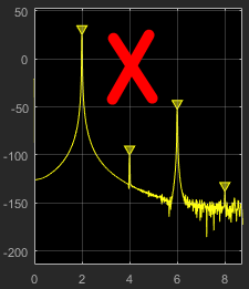
When you set the distortion Type to Intermodulation, the following fields appear in the Intermodulation Distortion panel at the bottom of the spectrum analyzer window.

F1 — Lower fundamental first-order frequency.
F2 — Upper fundamental first-order frequency.
2F1 - F2 — Lower intermodulation product from third-order harmonics.
2F2 - F1 — Upper intermodulation product from third-order harmonics.
TOI — Third-order intercept point. If the noise power is too high in relation to the harmonics, the TOI value will not be accurate. In this case, you should lower the resolution bandwidth or select a different spectral window. If the TOI has the same amplitude as the input two-tone signal, reduce the power of that input signal.

The intermodulation distortion measurement automatically locates the fundamental and the first-order frequencies (F1 and F2). It then computes the frequencies of the third-order intermodulation products (2F1−F2 and 2F2−F1).

For modifying the distortion measurements programmatically, see the DistortionMeasurementsConfiguration (DSP System Toolbox) object.

Channel Measurements

Measure the occupied bandwidth or adjacent channel power ratio (ACPR).

When you enable Channel Measurements, a channel measurements panel opens at the bottom of the spectrum analyzer window. This panel displays the occupied bandwidth or the adjacent channel power ratio measurements. Click the Channel Measurements drop-down arrow. You can specify the occupied bandwidth or the ACPR settings, frequency span, center frequency, and start and stop frequencies.

You can select the channel measurements Type to:

Occupied BW –– Occupied bandwidth
ACPR –– Ratio of the power of the main channel to the power of the adjacent channel

For more details on how the spectrum analyzer calculates the occupied bandwidth, see Occupied BW.

Occupied Bandwidth

When you set the channel measurements Type to Occupied BW, these fields appear in the measurements panel at the bottom of the scope window.

Channel Power (<%Spectrum Unit>) — Total power in the channel
Occupied BW (kHz) — Bandwidth containing the specified Occupied BW (%) of the total power of the spectrum.
Frequency Error (Hz) — Difference between the center of the occupied band and the center frequency (Center Frequency (Hz)) of the channel

ACPR

When you set the channel measurements Type to ACPR, these fields appear in the measurements panel at the bottom of the scope window.

Offset (kHz) — Frequency of adjacent channel relative to the center frequency of the main channel
Lower (Rel. Power (dBc)) — Ratio of the power of the lower sideband to the power of the main channel
Upper (Rel. Power (dBc)) — Ratio of the power of the upper sideband to the power of the main channel

To modify the channel measurements programmatically, see the ChannelMeasurementsConfiguration (DSP System Toolbox) object. For more information on these settings in the UI, see Channel Measurements.

Spectral Mask

Visualize spectrum limits and compare spectrum values to specification values.

Add upper and lower masks to the spectrum analyzer to visualize spectrum limits and compare spectrum values to specification values. When you enable the Spectral Mask on the Measurements tab, a Spectral Mask panel opens at the bottom of the spectrum analyzer window. Click the Upper Mask and Lower Mask parameters in the Spectral Mask drop-down to show the upper and lower masks, respectively. The Spectral Mask panel at the bottom of the spectrum analyzer window provides information on pass-fail statistics of masks, names of masks currently failing or passing, and names of channels causing the failure.

For more information on these settings in the UI, see Spectral Mask. For modifying the spectral mask measurements programmatically, see the SpectralMaskConfiguration (DSP System Toolbox) object.

Check Spectral Masks

You can check the status of the spectral mask using the getSpectralMaskStatus (DSP System Toolbox) function. This function gives details on the number of times a mask succeeded or failed, names of channels causing mask failure, and so on.

You can even use the MaskTestFailed event to perform an action every time the mask fails. To trigger a function when the mask fails, create a listener to the MaskTestFailed event and define a callback function to trigger it. For more details about using events, see Events.

Customize Visualization

Set configuration and style settings in the spectrum analyzer.

To control the settings of the display and labels, color and styling, click Display Settings () on the Home tab of the spectrum analyzer toolstrip.

In the dialog box that opens, you can customize the font size, plot type, y-axis properties of the spectrum plot, and color map properties of the spectrogram plot. You can change the color of the spectrum plot, background, axes, and labels and also change the line properties.

Display Controls

Use the display controls to:

Zoom and pan the axes.
Enable and disable the legend and the color bar.

To scale the plot axes, use the mouse to pan around the axes and the scroll button on your mouse to zoom in and out of the plot. Additionally, you can use the buttons that appear when you hover over the plot window.

— Maximize the axes, hide all labels and inset the axes values.
— Zoom in on the plot.
— Pan the plot.
— Autoscale the axes to fit the shown data.

To enable or disable the legend, click in the spectrum display.

To enable or disable the color bar, click in the spectrogram display.

Tips

If you set the Averaging Method to VBW or Exponential, and you introduce NaN or Inf values into the data, the spectrum appears blank. To ignore the NaN or Inf values:
- On the Home tab > Environment section of the MATLAB toolstrip, click Settings ().
- In the Workspace section of the Settings dialog box, select the Ignore NaNs when calculating statistics check box.
If you set Estimation Method to Filter bank in the block dialog box and click Step Back on the Simulink toolstrip, the spectrum analyzer uses data from the previous time step(s) to compute the spectrum in the current time step. This behavior leads to averaging the same data more than one time. To resolve this behavior, set Estimation Method to Welch and disable averaging. You can disable averaging using one of these settings:
- Set Averaging Method to Running and Spectral Averages to 1.
- Set Averaging Method to Exponential and Forgetting Factor to 0.

Algorithms

expand all

Spectrum Estimation — Filter Bank

When you choose the Filter Bank method, the spectrum analyzer uses an analysis filter bank to estimate the power spectrum. The filter bank contains a series of parallel bandpass filters that split an input broadband signal x(n), of sample rate fs, into multiple narrow band signals y₀(m), y₁(m), … , y_M-1(m), of sample rate fs/M so that each subband can be analyzed independently.

The variable M represents the number of frequency bands in the filter bank. In the spectrum analyzer, M is equal to the number of data points needed to achieve the specified RBW value or 1024, whichever is larger. For more information on the analysis filter bank and its implementation, see the More About (DSP System Toolbox) and the Algorithm (DSP System Toolbox) sections in the dsp.Channelizer object.

After the spectrum analyzer splits the broadband input signal into multiple narrow bands, it computes the power in each narrow frequency band using the following equation. Each Z_i value is the power estimate over that narrow frequency band.

$Z_{i} = \frac{1}{L} \sum_{m = 0}^{L - 1} {| y_{i} [m] |}^{2}$

L is length of the narrowband signal y_i(m) and i = 0, 1, …, M−1.

The power values in all the narrow frequency bands (denoted by Z_i) form the Z vector.

$Z = [Z_{0}, Z_{1}, Z_{2}, \dots, Z_{M - 1}]$

The spectrum analyzer averages the current Z vector with the previous Z vectors using one of the moving average methods: video bandwidth, exponential weighting, or running. The output of the averaging operation forms the spectral estimate vector. For details on the averaging methods, see Averaging Method.

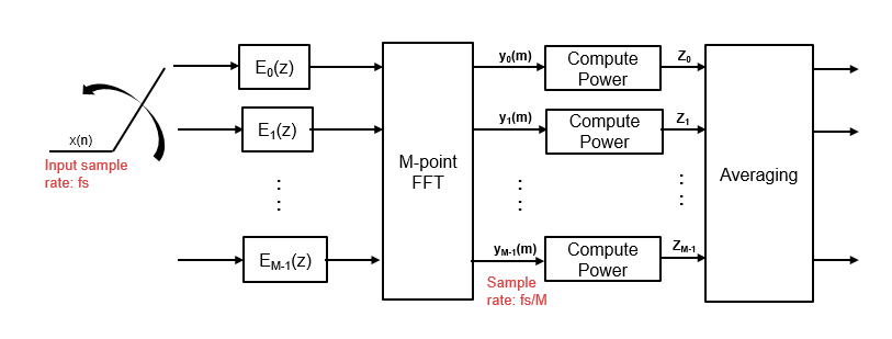
Input samples feed into polyphase branches. compute the M-point FFT of these polyphase branch outputs. Compute the power from the outputs and average the power.

The spectrum analyzer uses the value you specify in the RBW (Hz) parameter or the FFT Length parameter to determine the input frame length.

When you specify the Resolution Method to RBW, and you set RBW (Hz) to:

Auto –– The spectrum analyzer determines the appropriate resolution bandwidth to ensure that there are 1024 RBW intervals over the specified frequency span. When you set RBW (Hz) to Auto, the spectrum analyzer calculates RBW using this equation.
$R B W_{a u t o} = \frac{s p a n}{1024}$
scalar value –– The spectrum analyzer calculates the number of samples N_samples using this equation.

$N_{s a m p l e s} = \frac{F_{s}}{R B W}$
F_s is the sample rate of the input signal as specified in the Sample Rate (Hz) property.
The RBW value you specify must be such that there are at least two RBW intervals over the specified frequency span. The ratio of the overall span to RBW must be greater than two.
$\frac{s p a n}{R B W} > 2$
span is the frequency span over which the spectrum analyzer computes and plots the spectrum. To view the Span (Hz), on the Home tab on the spectrum analyzer toolstrip, click the Frequency Span drop-down arrow, and select the Span and Center Frequency.

When you specify the Resolution Method to Number of frequency bands, the resulting RBW is given by:

$R B W = \frac{F s}{F F T L e n g t h}$

When the number of input samples is not sufficient to achieve the specified resolution bandwidth, the spectrum analyzer adjusts its RBW value according to the number of input samples provided and displays a message similar to this one. The spectrum analyzer removes this message once you provide enough input samples.

Spectrum Estimation — Welch's Method

When you select the Welch method, the power spectrum estimate is the averaged modified periodograms.

The algorithm in the spectrum analyzer consists of these steps:

The block buffers the input into N-point data segments. Each data segment is split into P overlapping data segments, each of length M, overlapping by D points. The data segments can be represented as:

$\begin{array}{l} x_{i} (n) = x (n + i D), n = 0, 1, ..., M - 1 \\ i = 0, 1, ..., P - 1 \end{array}$
- If D = M/2, the overlap is 50%.
- If D = 0, the overlap is 0%.
Apply a window to each of the P overlapping data segments in the time domain.
If you set the Resolution Method to Window length, you can specify the data window length N_window using the Window Length parameter on the Estimation tab.
If you set the Resolution Method to RBW, the algorithm determines the data window length using this equation, $N_{w i n d o w} = \frac{N E N B W \times F s}{R B W}$ .
Then, it partitions the input signal into a number of windowed data segments.
Most window functions afford more influence to the data at the center of the set than to the data at the edges, which represents a loss of information. To mitigate that loss, the individual data sets are commonly overlapped in time. For each windowed segment, compute the periodogram by computing the discrete Fourier transform. Then compute the squared magnitude of the result and divide the result by M.

$P_{x x}^{i} (f) = \frac{1}{M U} {| \sum_{n = 0}^{M - 1} x_{i} (n) w (n) e^{- j 2 π f n} |}^{2}, i = 0, 1, ..., P - 1$
where U is the normalization factor for the power in the window function and is given by

$U = \frac{1}{M} \sum_{n = 0}^{M - 1} w^{2} (n)$
You can specify the window by clicking the Window drop-down arrow on the Estimation tab of the spectrum analyzer toolstrip.
The spectrum analyzer calculates and plots the power spectrum, power spectrum density, and RMS using the modified Periodogram estimator. For more information about the Periodogram method, see periodogram (Signal Processing Toolbox).
To determine the power spectrum estimate for Welch's method, the spectrum analyzer averages the result of the periodograms for the last P data segments. The averaging reduces the variance, compared to the original N-point data segment. For more details on the averaging, see Averaging Method.

$PSD (f) = \frac{1}{P} \sum_{i = 0}^{P - 1} P_{x x}^{i} (f)$
- The spectrum analyzer computes the power spectral density using:
  
  $PSD (f) = \frac{1}{P * F_{s}} \sum_{i = 0}^{P - 1} P_{x x}^{i} (f)$
- The power spectrum is the product of the power spectral density and the resolution bandwidth, as given by this equation.
  $P_{s p e c t r u m} (f) = PSD (f) \times R B W = PSD (f) \times \frac{F_{s} \times N E N B W}{N_{w i n d o w}}$

The spectrum analyzer uses a certain number of samples to compute a spectral estimate. This value is directly related to the resolution bandwidth (RBW) using this equation, $N_{s a m p l e s} = \frac{(1 - \frac{O_{p}}{100}) \times N E N B W \times F_{s}}{R B W},$

where O_p is the overlap percentage, NENBW is the normalized effective noise bandwidth, F_s is the input sample rate, and RBW is the resolution bandwidth.

The spectrum analyzer shows the number of samples per update in the spectrum analyzer status bar. Click the $⋮$ icon in the status bar and select Samples/Update (S/U).

When you specify the Resolution Method to RBW, the window length is given by,

$N_{w i n d o w} = \frac{N E N B W \times F_{s}}{R B W}$

When you specify the Resolution Method to Window length, the algorithm uses the window length value you specify in the Window Length parameter on the Estimation tab on the spectrum analyzer toolstrip.

Overlap Percentage (O_p)

The overlap percentage O_p is the value you specify in the Overlap % property. To view the Overlap % parameter, on the Estimation tab on the spectrum analyzer toolstrip, click the Window drop-down arrow.

When you increase the overlap percentage, the spectrum analyzer needs fewer new input samples to compute a new spectral update.

O_p	N_samples
0%	100
50%	50
80%	20

Normalized Effective Noise Bandwidth (NENBW)

The normalized effective noise bandwidth NENBW is a window parameter that measures the noise performance of the window. NENBW is determined using the window length and the window coefficients, and is given by the following equation:

$N E N B W = N_{w i n d o w} \times \frac{\sum_{n = 1}^{N_{w i n d o w}} w^{2} (n)}{{[\sum_{n = 1}^{N_{w i n d o w}} w (n)]}^{2}},$

w(n) denotes the vector of window coefficients. N_window is the window length. For more information on how the algorithm determines the window length, see the Spectrum Estimation –– Welch's Method section in Algorithms.

The rectangular window has the smallest NENBW, with a value of 1. All other windows have a larger NENBW value. For example, the Hann window has an NENBW value of approximately 1.5.

The spectrum analyzer shows the value of NENBW in the spectrum analyzer status bar. Click the $⋮$ icon in the status bar and select NENBW.

Input Sample Rate (Fs)

F_s is the sample rate of the input signal. You can view the Sample Rate (Hz) on the Home tab of the spectrum analyzer toolstrip. You can enable this property in the status bar at the bottom of the spectrum analyzer window. Click the icon in the status bar and select Sample Rate (Fs).

Resolution Bandwidth (RBW)

Resolution bandwidth controls the spectral resolution of the displayed signal. The RBW value determines the spacing between frequencies that the scope can resolve. A smaller value gives a higher spectral resolution and lowers the noise floor, that is, the spectrum analyzer can resolve frequencies that are closer to each other. However, this comes at the cost of a longer sweep time.

You can specify the resolution bandwidth using the RBW (Hz) parameter.

If you specify the window length, the scope determines the RBW value from the window length using this equation, $R B W = \frac{N E N B W \times F s}{N_{w i n d o w}},$ .

When you specify the Resolution Method to RBW, and you set RBW (Hz) to:

Auto –– The spectrum analyzer determines the appropriate resolution bandwidth to ensure that there are 1024 RBW intervals over the specified frequency span. When you set RBW (Hz) to Auto, the spectrum analyzer calculates using this equation.
$R B W_{a u t o} = \frac{s p a n}{1024}$
scalar value –– Specify a value such that there are at least two RBW intervals over the specified frequency span. The ratio of the overall span to RBW must be greater than two:
$\frac{s p a n}{R B W} > 2$

span is the frequency span over which the spectrum analyzer computes and plots the spectrum. Spectrum analyzer shows the span through the Span (Hz) property.

When you specify the Resolution Method to Number of frequency bands, the resulting RBW is given by:

$R B W = \frac{F s}{F F T L e n g t h}$

You can enable this property in the status bar at the bottom of the spectrum analyzer window. Click the icon in the status bar and select RBW.

Nyquist Frequency Interval

When you plot the two-sided spectrum by selecting Two-Sided Spectrum in the Frequency Span options, the Nyquist frequency interval is $[- \frac{S a m p l e R a t e}{2}, \frac{S a m p l e R a t e}{2}] + F r e q u e n c y O f f s e t$ Hz.

When you clear the Two-Sided Spectrum, the Nyquist frequency interval is $[0, \frac{S a m p l e R a t e}{2}] + F r e q u e n c y O f f s e t$ Hz.

Frequency Vector

When you select the Auto Frequency Vector under the Frequency Span options, the software calculates the frequency vector for the frequency-domain input.

When you plot the two-sided spectrum by selecting Two-Sided Spectrum in the Frequency Span options, the frequency vector is:

$[- \frac{S a m p l e R a t e}{2}, \frac{S a m p l e R a t e}{2}]$

When you clear the Two-Sided Spectrum, the frequency vector is:

$[0, \frac{S a m p l e R a t e}{2}]$

Occupied BW

The spectrum analyzer calculates Occupied BW using these steps.

Calculate the total power in the measured frequency range.
Determine the lower frequency value. Starting at the lowest frequency in the range and moving upward, sum the power distributed in each frequency until the result is

$\frac{100 - O c c u p i e d B W %}{2}$
of the total power.
Determine the upper frequency value. Starting at the highest frequency in the range and moving downward, sum the power distributed in each frequency until the result reaches

$\frac{100 - O c c u p i e d B W %}{2}$
of the total power.
The bandwidth between the lower and upper power frequency values is the occupied bandwidth.
The frequency halfway between the lower and upper frequency values is the center frequency.

Distortion Measurements

The spectrum analyzer calculates Distortion Measurements using these steps.

Estimate spectral content by finding peaks in the spectrum. When the algorithm detects a peak, it records the width of the peak and clears all monotonically decreasing values by treating all these values as if they belong to the peak. Using this method, the algorithm removes all spectral content centered at DC (0 Hz) from the spectrum and records the amount of bandwidth cleared (W₀).
Determine the fundamental power (P₁) from the remaining maximum value of the displayed spectrum. Create a local estimate (Fe₁) of the fundamental frequency by computing the central moment of the power near the peak. Record the bandwidth of the fundamental power content (W₁). Then remove the power from the fundamental as in step 1.
Determine the power and width of the higher-order harmonics (P₂, W₂, P₃, W₃, etc.) in succession by examining the frequencies closest to the appropriate multiple of the local estimate (Fe₁). Remove any spectral content that decreases monotonically about the harmonic frequency from the spectrum before proceeding to the next harmonic.
After removing the DC, fundamental, and harmonic content from the spectrum, examine the power of the remaining spectrum for its sum (P_remaining), peak value (P_maxspur), and median value (P_estnoise).
Compute the sum of all the removed bandwidth as W_sum = W₀ + W₁ + W₂ +...+ W_n.
Compute the sum of powers of the second and higher-order harmonics as P_harmonic = P₂ + P₃ + P₄ +...+ P_n.
Estimate the sum of the noise power as:
$P_{n o i s e} = (P_{r e m a i n i n g} \cdot d F + P_{e s t . n o i s e} \cdot W_{s u m}) / R B W$
Where dF is the absolute difference between frequency bins, and RBW is the resolution bandwidth of the window.
Then compute the metrics for THD, THD%, SINAD, SNR, and SFDR from the estimates.

$\begin{array}{l} T H D = 10 \cdot \log_{10} (\frac{P_{h a r m o n i c}}{P_{1}}) \\ T H D % = 100 \cdot 10^{(T H D / 20)} \\ S I N A D = 10 \cdot \log_{10} (\frac{P_{1}}{P_{h a r m o n i c} + P_{n o i s e}}) \\ S N R = 10 \cdot \log_{10} (\frac{P_{1}}{P_{n o i s e}}) \\ S F D R = 10 \cdot \log_{10} (\frac{P_{1}}{\max (P_{m a x s p u r}, \max (P_{2}, P_{3}, ..., P_{n}))}) \end{array}$

Harmonic Measurements

The harmonic distortion measurements use the spectrum trace shown in the display as the input to the measurements. The default Hann window setting of the spectrum analyzer might exhibit leakage that can completely mask the noise floor of the measured signal.
The harmonic measurements attempt to correct for leakage by ignoring all frequency content that decreases monotonically away from the maximum of harmonic peaks. If the window leakage covers more than 70% of the frequency bandwidth in your spectrum, you may see a blank reading (–) reported for SNR and SINAD. If your application can tolerate the increased equivalent noise bandwidth (ENBW), consider using a Kaiser window with a high attenuation (up to 300 dB) to minimize spectral leakage.
Ignore the DC component.
After windowing, the width of each harmonic component masks the noise power in the neighborhood of the fundamental frequency and harmonics. To estimate the noise power in each region, the spectrum analyzer computes the median noise level in the nonharmonic areas of the spectrum. It then extrapolates that value into each region.
N^th order intermodulation products occur at A*F1 + B*F2,
where F1 and F2 are the sinusoid input frequencies and |A| + |B| = N. A and B are integer values.
For intermodulation measurements, compute the third-order intercept (TOI) point as follows.
- TOI_lower = P_F1 + (P_F2 - P_(2F1-F2))/2
- TOI_upper = P_F2 + (P_F1 - P_(2F2-F1))/2
- TOI = (TOI_lower + TOI_upper)/2
Where P is power in decibels of the measured power referenced to 1 milliwatt (dBm).

Averaging Method

The spectrum analyzer calculates the moving average using one of these methods:

Video bandwidth — The spectrum analyzer uses a time-domain lowpass filter to smooth the noise in the signal. The video bandwidth (VBW) filter smoothes the trace and decreases noise, and the spectrum analyzer applies the filter to the data before displaying it.
Video bandwidth is the bandwidth of the lowpass filter that spectrum analyzer uses to average or smooth the noise in the signal before displaying it in the scope. The spectrum analyzer computes the video bandwidth using this equation:

$V B W = \frac{(1 - λ) R B W}{2 π λ N E N B W}$
where,
- λ is the forgetting factor.
- RBW is the resolution bandwidth.
- NENBW is the normalized effective noise bandwidth.
Video bandwidth does not affect the level of the noise (noise floor), but only increases the signal-to-noise ratio and smoothes the trace of the noise. When you decrease the value of VBW, the signal-to-noise ratio improves.
The cutoff frequency of the video bandwidth filter is given by:

$ω_{c} = \frac{2 π V B W}{F_{s} / N F F T}$
where Fs is the input sample rate and NFFT is the number of FFT points.
The spectrum analyzer shows the values of sample rate, VBW, and NFFT in the status bar at the bottom of the display. To enable, right-click the status bar and select Sample Rate (Fs), VBW, and FFT Length (NFFT).
Exponential — The moving average algorithm uses the exponential weighting method to update the weights and compute the moving average recursively for each Z vector that comes in by using the following recursive equations:
$\begin{array}{l} w_{N} = λ w_{N - 1} + 1 \\ {\bar{z}}_{N} = (1 - \frac{1}{w_{N}}) {\bar{z}}_{N - 1} + (\frac{1}{w_{N}}) z_{N} \end{array}$
- λ — Forgetting factor
- $w_{N}$ — Weighting factor applied to the current Z vector
- $z_{N}$ — Current Z vector
- ${\bar{z}}_{N - 1}$ — Moving average until the previous Z vector
- $(1 - \frac{1}{w_{N}}) {\bar{z}}_{N - 1}$ — Effect of the previous Z vectors on the average
- ${\bar{z}}_{N}$ — Moving average including the current Z vector
Running –– For each frame of the input, average the last Q scaled Z vectors, which are computed by the algorithm. The variable Q is the value you specify for the number of spectral averages. If the algorithm does not have enough Z vectors, the algorithm uses zeros to fill the empty elements.

Extended Capabilities

expand all

C/C++ Code Generation
Generate C and C++ code using Simulink® Coder™.

This block can be used for simulation visibility in systems that generate code, but is not included in the generated code.

HDL Code Generation
Generate VHDL, Verilog and SystemVerilog code for FPGA and ASIC designs using HDL Coder™.

HDL Coder™ provides additional configuration options that affect HDL implementation and synthesized logic. See also Add Comments to Generated HDL Code (HDL Coder) and Integrate Custom HDL Code by Using DocBlock (HDL Coder).

HDL Architecture

Architecture	Description
`No HDL`	Do not generate HDL code for this block.

HDL Block Properties

PreserveUpstreamLogic

Control the removal of unconnected logic. The default is off, which means unconnected logic is not preserved in HDL code. For more details, see PreserveUpstreamLogic (HDL Coder).

PLC Code Generation
Generate Structured Text code using Simulink® PLC Coder™.

This block can be used for simulation visibility in systems that generate PLC code, but is not included in the generated code.

Version History

Introduced in R2014b

expand all

R2026b: New streamlined user interface in spectrum analyzer

The spectrum analyzer toolstrip is reorganized into these three tabs to give you easy and streamlined access to the scope settings.

The Home tab contains all the general settings for the spectrum and spectrogram display.
The Estimation tab contains settings that control the frequency resolution and spectral averaging.
The Measurements tab contains settings to control the measurements supported by the scope.

R2026b: New Print to Figure export option

Print the scope display to a MATLAB figure by clicking the Print to Figure option on the Home tab > Export section.

R2026b: Enhancements to spectrum analyzer status bar

The spectrum analyzer status bar has these enhancements:

New dB Full Scale (dBFS) parameter that shows the dB full scale value.

Certain parameter names have changed and some of the parameters have new readouts in the status bar. For more information, see the following table.

Status Bar Parameter in R2026a or Earlier	Status Bar Parameter in R2026b	Status Bar Readout in R2026b
`Sample Rate`	`Sample Rate (Fs)`	`Fs`
`Samples/Update`	`Samples/Update (S/U)`	`S/U`
`Time Resolution`	`Time Resolution (ΔT)`	`ΔT`
`NFFT`	`FFT Length (NFFT)`	`NFFT`
`Forgetting Factor`	`Forgetting Factor (α)`	`α`
`Spectral Averages`	`Spectral Averages (Navg)`	`Navg`
—	`dB Full Scale (dBFS)`	`dBFS`

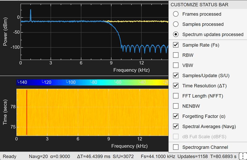
Spectrum analyzer showing the status bar with new readouts.

R2026b: Set Window Length to `Auto`

You can set the Window Length parameter to Auto or to an integer greater than 2. In the Auto setting, the scope uses the frame length of the first input as the window length.

R2026a: Support for horizontal spectrogram scrolling

You can now switch the time orientation of the spectrogram in the Spectrum Analyzer block from the default vertical direction to the horizontal direction using the Time Orientation parameter. With this change, as the simulation time progresses, the spectrogram moves in the horizontal direction from right to left.

R2026a: Autoscaling of axes limits

You can now automatically scale the y-axis limits of the spectrum analyzer display and the color limits of the spectrogram by selecting the Automatically Scale Axes Limits parameter. If you clear this parameter, use the Y-Limits and the Color Limits parameters to manually scale the axes limits.

R2025a: Control plot type for each line individually

You can now individually control the type of plot for each line. To control the type of plot for a line, select the line and set the Plot Type parameter accordingly.

R2025a: New phase noise measurements in Spectrum Analyzer block

You can now measure and plot the phase noise of a signal using the Spectrum Analyzer block.

To enable the phase noise measurements in the Spectrum Analyzer window, click the Measurements tab on the scope toolstrip and then click the Phase Noise button.

Note

To access the phase noise measurement settings, you must have a valid Mixed-Signal Blockset license.

R2025a: Support for running averaging method

The Spectrum Analyzer block now supports the running averaging method to compute the power spectrum estimate. To enable this mode, set the Averaging Method parameter on the Estimation tab to Running and the Spectral Averages parameter to a positive integer.

For more information, see the Algorithms section.

R2024b: Display spectral data for any number of input samples and adjust RBW accordingly

Previously, the Spectrum Analyzer block required a minimum number of samples to update the display for a given RBW value. Starting in R2024b, this limitation is removed. The scope now updates its display for any number of input samples and adjusts the RBW value accordingly.

R2024b: Auto adjust RBW to maintain 1024 samples

The Spectrum Analyzer block can now automatically adjust the resolution bandwidth (RBW) so as to maintain the number of samples per spectral update at 1024 (Nsamples = 1024) irrespective of the window you select.

To enable this mode in the Spectrum Analyzer block, set:

RBW (Hz) to Auto.

R2024b: Higher display precision in scope UI

You can now increase the display precision to 15 digits using the Display Precision property in the scope settings under Display and Labels. This precision affects all the measurements and data that the scope displays on its status bar.

R2024b: Preserve Colors is now available in scope toolstrip

The Preserve colors for copy to clipboard property has been renamed to Preserve Colors and is now available in the scope toolstrip under Copy Display.

R2024a: Analyzer tab has been renamed as Scope tab

The Analyzer tab in spectrum analyzer has been renamed as Scope tab.

R2024a: Specify window length and FFT length

You can now specify the window length and FFT length in the spectrum analyzer under certain conditions. These parameters are available starting R2024a:

Resolution Method
Window Length
FFT Length

R2023b: Spectrum Analyzer supports `dBuV` units

You can set Spectrum Unit to dBuV when you set:

Input Domain to Time and Spectrum to RMS.
Input Domain to Frequency.

You can set Input Unit to dBuV when you set Input Domain to Frequency.

R2023a: Spectrum Analyzer with improved responsiveness and toolstrip interface in Simulink

In R2023a, the Spectrum Analyzer block is more responsive and its toolstrip interface is improved to provide you easy access to spectral analysis, estimation, and measurements. You can configure and display Spectrum Analyzer settings from the command line with the SpectrumAnalyzerBlockConfiguration (DSP System Toolbox) object.

Spectrum Analyzer

Description

Measurements

Programmatic Control

Examples

Display Frequency Input on Spectrum Analyzer

Display Variable-Size Input Signals on Spectrum Analyzer

Obtain Measurements Data Programmatically for Spectrum Analyzer Block

Extended Examples

Spectrum Analyzer Measurements

High Resolution Spectral Analysis in Simulink

Ports

Input

u — Signals to visualize scalar | vector | matrix | array

F — Frequencies in Hz column vector

Dependencies

RBW — RBW Value positive scalar

Dependencies

VBW — VBW Value positive scalar

Dependencies

Parameters

Home Tab

Views

Spectrum — Enable spectrum display button

Trace Settings

Normal Trace — Plot power spectral estimate on (default) | off

Dependencies

Programmatic Use

Max-Hold Trace — Plot running maximum of power spectral estimate off (default) | on

Dependencies

Programmatic Use

Min-Hold Trace — Plot running minimum of power spectral estimate off (default) | on

Dependencies

Programmatic Use

Spectrogram — Enable spectrogram display button

Channel and Time Settings

Spectrogram Channel — Channel for which spectrogram is plotted 1 (default) | character vector of a positive integer | string scalar of a positive integer

Programmatic Use

Auto Time Span — Enable auto time span on (default) | off

Programmatic Use

Time Span (s) — Time span in seconds positive scalar

Dependencies

Programmatic Use

Auto Time Resolution — Enable auto time resolution on (default) | off

Programmatic Use

Time Resolution (s) — Time resolution in seconds positive scalar

Dependencies

Programmatic Use

Vertical Scrolling — Enable vertical orientation of time in spectrogram on (default) | off

Programmatic Use

Display Settings — Set configuration and style settings button

Display Settings

Num Inputs — Number of input ports 1 (default) | integer between 1 and 96

Programmatic Use

Open at Simulation Start — Automatically open scope when simulation starts on (default) | off

Programmatic Use

Title — Display title character vector | string

Programmatic Use

Y-Label — y-axis label character vector | string scalar

Dependencies

Programmatic Use

Display Precision — Precision of data in scope display 4 (default) | positive integer ≤ 15

Show Grid — Show internal grid lines on (default) | off

Programmatic Use

Automatically Scale Axes Limits — Option to automatically scale y-axis limits and color limits on (default) | off

Programmatic Use

Y-Limits — y-axis limits [−80 20] | [ymin ymax]

Dependencies

Programmatic Use

Color Limits — Color limits of spectrogram [-80 20] (default) | [colorMin colorMax]

Dependencies

Programmatic Use

Color Map — Spectrogram colormap jet (default) | hot | bone | cool | copper | gray | parula | three-column matrix

Dependencies

Programmatic Use

Layout — Stack axes vertically or horizontally Vertical (default) | Horizontal

Dependencies

Programmatic Use

Font Size — Font size of labels 8.5 (default) | positive scalar

Background Color — Window background black (default) | color picker

u — Signals to visualize
scalar | vector | matrix | array

F — Frequencies in Hz
column vector

RBW — RBW Value
positive scalar

VBW — VBW Value
positive scalar

Spectrum — Enable spectrum display
button

Normal Trace — Plot power spectral estimate
`on` (default) | `off`

Max-Hold Trace — Plot running maximum of power spectral estimate
`off` (default) | `on`

Min-Hold Trace — Plot running minimum of power spectral estimate
`off` (default) | `on`

Spectrogram — Enable spectrogram display
button

Spectrogram Channel — Channel for which spectrogram is plotted
`1` (default) | character vector of a positive integer | string scalar of a positive integer

Auto Time Span — Enable auto time span
`on` (default) | `off`

Time Span (s) — Time span in seconds
positive scalar

Auto Time Resolution — Enable auto time resolution
`on` (default) | `off`

Time Resolution (s) — Time resolution in seconds
positive scalar

Vertical Scrolling — Enable vertical orientation of time in spectrogram
`on` (default) | `off`

Display Settings — Set configuration and style settings
button

Num Inputs — Number of input ports
1 (default) | integer between 1 and 96

Open at Simulation Start — Automatically open scope when simulation starts
`on` (default) | `off`

Title — Display title
character vector | string

Y-Label — y-axis label
character vector | string scalar

Display Precision — Precision of data in scope display
`4` (default) | positive integer ≤ 15

Show Grid — Show internal grid lines
`on` (default) | `off`

Automatically Scale Axes Limits — Option to automatically scale y-axis limits and color limits
`on` (default) | `off`

Y-Limits — y-axis limits
[`−80` `20`] | [`ymin ymax`]

Color Limits — Color limits of spectrogram
[`-80 20`] (default) | [`colorMin colorMax`]

Color Map — Spectrogram colormap
`jet` (default) | `hot` | `bone` | `cool` | `copper` | `gray` | `parula` | three-column matrix

Layout — Stack axes vertically or horizontally
`Vertical` (default) | `Horizontal`

Font Size — Font size of labels
`8.5` (default) | positive scalar

Background Color — Window background
black (default) | color picker

Axes Color — Axes background color
black (default) | color picker

Labels Color — Color of labels
gray (default) | color picker

Line Selector — Channel for line property settings
channel names

Plot Type — Plot type
`Line` (default) | `Stem`

Line Visible — Channel visibility
`on` (default) | `off`

Line Style — Line style
`-` (default) | `:` | `-`. | `--` | `None`

Line Width — Line width
`1.5` (default) | `0.5` | `1` | `2` | ...

Line Marker — Data point markers
`None` (default) | `+` | `x` | ...

Line Color — Line color
yellow (default) | color picker

Input Domain — Domain of the input signal
`Time` (default) | `Frequency`

Sample Rate (Hz) — Sample rate the scope uses in Hz
`Inherited` (default) | positive scalar

Frequency Scale — Scale of frequency axis
`Linear` (default) | `Log`

Frequency Span — Frequency span settings
drop-down

Two-Sided Spectrum — Show two-sided spectrum
`on` (default) | `off`

Frequency Span — Frequency span mode
Full (default) | Span and Center Frequency | Start and Stop Frequencies

Span (Hz) — Frequency span to compute spectrum in Hz
`10e3` (default) | real positive scalar

Center Frequency (Hz) — Center of frequency span in Hz
`0` (default) | real scalar

Start Frequency (Hz) — Start frequency in Hz
`-5e3` (default) | scalar

Stop Frequency (Hz) — Stop frequency in Hz
`5e3` (default) | scalar

Frequency Vector — Frequency vector source
Auto Frequency Vector (default) | Input Frequency Vector | Specify Frequency Vector

Frequency Vector (Hz) — Custom frequency vector
[`-5e3 5e3`] (default) | monotonically increasing vector

Frequency Offset (Hz) — Offset to apply to frequency axis
`0` (default) | scalar | vector

Spectrum Type — Type of spectrum or spectrogram to display
`Power` (default) | `Power Density` | `RMS`

Spectrum Unit — Units of the spectrum
`dBm` (default) | `dBFS` | `dBV` | `dBuV` (since R2023b) | `dBW` | `Vrms` | `Watts` | `dBm/Hz` | `dBW/Hz` | `dBFS/Hz` | `Watts/Hz` | `Auto`

Input Unit — Units of frequency input
`dBm` (default) | `dBuV` (since R2023b) | `dBV` | `dBW` | `Vrms` | `Watts` | `None`

Scale — Scale options
drop-down

Auto dB Full Scale — Enable auto dB full scale
`on` (default) | `off`

dB Full Scale — Specify full scale value in dB
`1` (default) | positive real scalar