Two Cylinder Model with Load Constraints
This example shows how to model a rigid rod supporting a large mass interconnecting two hydraulic actuators. This model eliminates the springs as it applies the piston forces directly to the load. These forces balance the gravitational force and result in both linear and rotational displacement.
Model Analysis and Physics
The rotation angle of the rod is small. The equations of motion for the rod are given below in Equation Set 1. The equations describing the cylinder and pump behavior are the same as in the single cylinder example.
Equation Set 1:


The positions and velocities of the individual pistons follow directly from the geometry. See the corresponding equations in Equation Set 2.
Equation Set 2:


Opening and Simulating Model
To open this model, type this command: sldemo_hydrod. To run the simulation, on the Simulation Toolstrip, click Run. The model:
Logs signal data to the MATLAB® workspace in the
Simulink.SimulationOutputobjectout. The signal logging data is stored inout, in aSimulink.SimulationData.Datasetobject calledsldemo_hydrod_output.
Logs continuous states data to MATLAB workspace. The states data is also contained in the
outworkspace variable, as a structure calledxout. Each state is assigned a name in the model to help working with logged data. The names of the states are available in thestateNamefield ofxout.signals. For more information, see Data Format for Logged Simulation Data.
Uses the customizable Circular Gauge and Vertical Gauge blocks to visualize the fluid flow, pressure, and linear displacement in the cylinders.

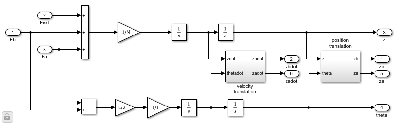
Mechanical Load Subsystem
The Mechanical Load subsystem solves the equations of motion, which are computed directly using standard Simulink blocks. The rotation angle is assumed to be small. To look under the mask of the Mechanical Load subsystem and see its structure, right-click the subsystem and select Edit Mask > Look Under Mask.
Simulation Parameters
The parameters used in this simulation are identical to the parameters used in the Single Hydraulic Cylinder Simulation model, except for the following:
L     = 1.5 m
M     = 2500 kg
I     = 100 kg/m^2
Qmax = 0.005 m^3/sec (constant)
C2    = 3e-9 m^3/sec/Pa
Fext  = -9.81*M Newtons
Although the pump flow is constant, the model controls the valves independently. Initially, at t = 0, the cross-section of valve B is zero. The value grows linearly to 1.2e-5 m^2 at t = 0.01 sec, and then linearly decreases to zero at t = 0.02 sec. The cross-section of valve A is 1.2e-5 sq.m. at t = 0. The value linearly decreases to zero at t = 0.01 sec, and then it linearly increases to 1.2e-5 sq.m. at t = 0.02 sec. Then the behavior of the valves A and B repeats periodically with the same pattern. In other words, the valves A and B are 180 degrees out of phase.
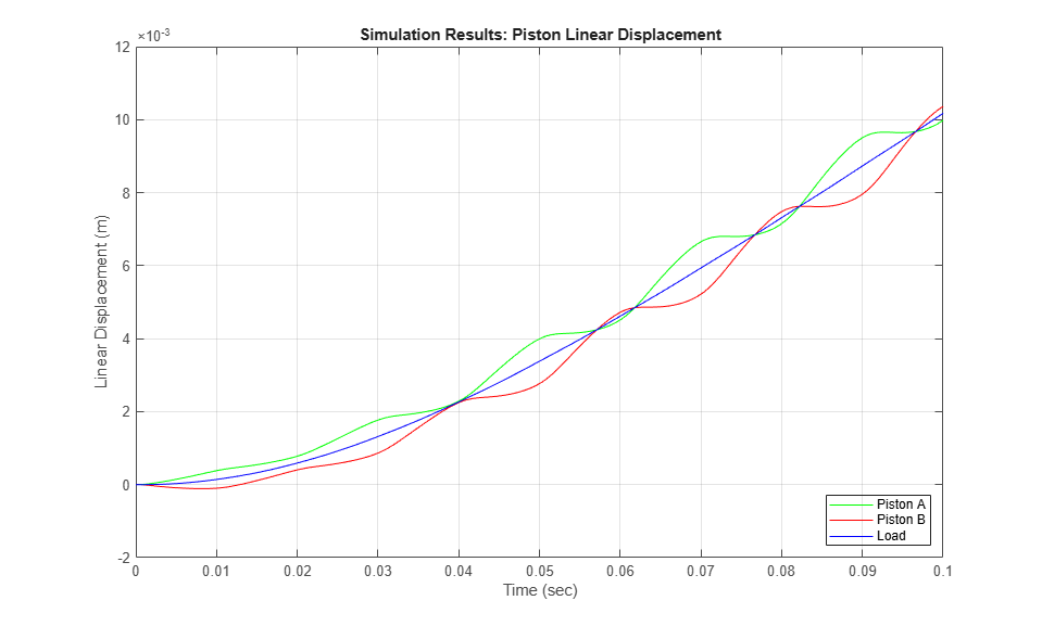
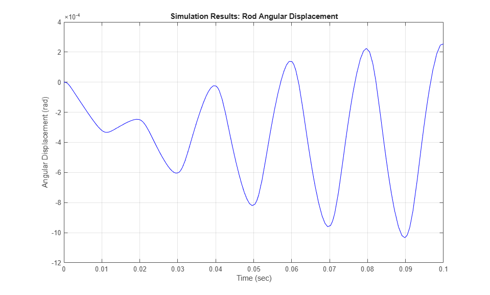
Results
These plots show the linear and angular displacements of the rod. The linear displacement response is typical of a type-one integrating system. The relative positions and the angular movement of the rod illustrate the response of the two pistons to the out-of-phase control signals, or the cross-section of the valves A and B.