Batch Linearize Model at Multiple Operating Points Derived from Parameter Variations
If your application includes parameter variations that affect the operating point of the model, you must batch trim the model for the parameter variations before linearization. Use this batch linearization approach when computing linear models for linear parameter-varying systems.
For more information on batch trimming models for parameter variations, see Batch Compute Steady-State Operating Points for Parameter Variation.
Open the Simulink® model.
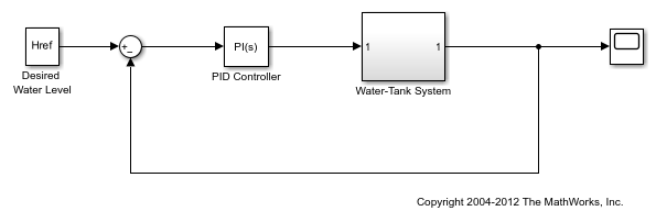
sys = 'watertank';
open_system(sys)
Vary parameters A and b within 10% of their nominal values. Specify three values for A and four values for b, creating a 3-by-4 value grid for each parameter.
[A_grid,b_grid] = ndgrid(linspace(0.9*A,1.1*A,3),...
                         linspace(0.9*b,1.1*b,4));
Create a parameter structure array, specifying the name and grid points for each parameter.
params(1).Name = 'A';
params(1).Value = A_grid;
params(2).Name = 'b';
params(2).Value = b_grid;
Create a default operating point specification for the mode that specifies that both model states are unknown and must be at steady state in the trimmed operating point.
opspec = operspec(sys);
Trim the model using the specified operating point specification, parameter grid, and option set. Suppress the display of the operating point search report.
opt = findopOptions('DisplayReport','off');
[op,opreport] = findop(sys,opspec,params,opt);
findop trims the model for each parameter combination using only one model compilation. op is a 3-by-4 array of operating point objects that correspond to the specified parameter grid points.
To compute the closed-loop input/output transfer function for the model, define the linearization input and output points as the reference input and model output, respectively.
io(1) = linio('watertank/Desired  Water Level',1,'input');
io(2) = linio('watertank/Water-Tank System',1,'output');
To extract multiple open-loop and closed-loop transfer functions from the same model, batch linearize the system using an slLinearizer interface. For more information, see Vary Parameter Values and Obtain Multiple Transfer Functions.
Batch linearize the model at the trimmed operating points using the specified I/O points and parameter variations.
G = linearize(sys,op,io,params);
G is a 3-by-4 array of linearized models. Each entry in the array contains a linearization for the corresponding parameter combination in params. For example, G(:,:,2,3) corresponds to the linearization obtained by setting the values of the A and b parameters to A_grid(2,3) and b_grid(2,3), respectively. The set of parameter values corresponding to each entry in the model array G is stored in the SamplingGrid property of G. For example, examine the corresponding parameter values for linearization G(:,:,2,3):
G(:,:,2,3).SamplingGrid
ans =

  struct with fields:

    A: 20
    b: 5.1667
When batch linearizing for parameter variations, you can obtain the linearization offsets that correspond to the linearization operating points. To do so, set the StoreOffsets linearization option.
opt = linearizeOptions('StoreOffsets',true);
Linearize the model using the specified parameter grid, and return the linearization offsets in the info structure.
[G,~,info] = linearize('watertank',io,params,opt);
You can then use the offsets to configure an LPV System block. To do so, you must first convert the offsets to the required format. For an example, see LPV Approximation of Boost Converter Model.
offsets = getOffsetsForLPV(info);
See Also
linearize | linio | findop | ndgrid