Digital Control of Power Stage Voltage
This example shows how to tune a high-performance digital controller with bandwidth close to the sampling frequency.
Voltage Regulation in Power Stage
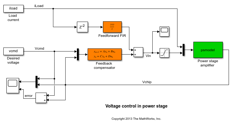
We use Simulink® to model the voltage controller in the power stage for an electronic device:
open_system('rct_powerstage')
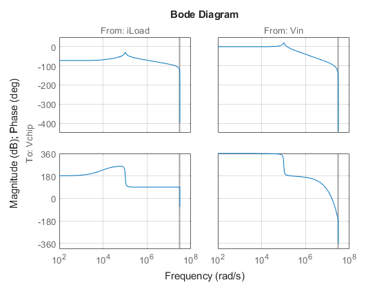
The power stage amplifier is modeled as a second-order linear system with the following frequency response:
bode(psmodel)
grid
The controller must regulate the voltage Vchip delivered to the device to track the setpoint Vcmd and be insensitive to variations in load current iLoad. The control structure consists of a feedback compensator and a disturbance feedforward compensator. The voltage Vin going into the amplifier is limited to  . The controller sampling rate is 10 MHz (sample time
 Tm is 1e-7 seconds).
Performance Requirements
This application is challenging because the controller bandwidth must approach the Nyquist frequency pi/Tm = 31.4 MHz. To avoid aliasing troubles when discretizing continuous-time controllers, it is preferable to tune the controller directly in discrete time.
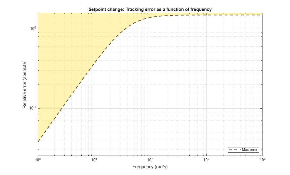
The power stage should respond to a setpoint change in desired voltage Vcmd in about 5 sampling periods with a peak error (across frequency) of 50%. Use a tracking requirement to capture this objective.
Req1 = TuningGoal.Tracking('Vcmd','Vchip',5*Tm,0,1.5);
Req1.Name = 'Setpoint change';

viewGoal(Req1)
The power stage should also quickly reject load disturbances iLoad. Express this requirement in terms of gain from iLoad to Vchip. This gain should be low at low frequency for good disturbance rejection.
s = tf('s');
nf = pi/Tm;   % Nyquist frequency

Req2 = TuningGoal.Gain('iLoad','Vchip',1.5e-3 * s/nf);
Req2.Focus = [nf/1e4, nf];
Req2.Name = 'Load disturbance';
High-performance demands may lead to high control effort and saturation. For the ramp profile vcmd specified in the Simulink model (from 0 to 1 in about 250 sampling periods), we want to avoid hitting the saturation constraint  . Use a rate-limiting filter to model the ramp command, and require that the gain from the rate-limiter input to
  be less than
  .
.
RateLimiter = 1/(250*Tm*s); % models ramp command in Simulink

% |RateLimiter * (Vcmd->Vin)| < Vmax
Req3 = TuningGoal.Gain('Vcmd','Vin',Vmax/RateLimiter);
Req3.Focus = [nf/1000, nf];
Req3.Name = 'Saturation';
To ensure adequate robustness, require at least 7 dB gain margin and 45 degrees phase margin at the plant input.
Req4 = TuningGoal.Margins('Vin',7,45);
Req4.Name = 'Margins';
Finally, the feedback compensator has a tendency to cancel the plant resonance by notching it out. Such plant inversion may lead to poor results when the resonant frequency is not exactly known or subject to variations. To prevent this, impose a minimum closed-loop damping of 0.5 to actively damp of the plant's resonant mode.
Req5 = TuningGoal.Poles(0,0.5,3*nf);
Req5.Name = 'Damping';
Tuning
Next use systune to tune the controller parameters subject to the requirements defined above. First use the slTuner interface to configure the Simulink model for tuning. In particular, specify that there are two tunable blocks and that the model should be linearized and tuned at the sample time Tm.
TunedBlocks = {'compensator','FIR'};
ST0 = slTuner('rct_powerstage',TunedBlocks);
ST0.Ts = Tm;

% Register points of interest for open- and closed-loop analysis
addPoint(ST0,{'Vcmd','iLoad','Vchip','Vin'});
We want to use an FIR filter as feedforward compensator. To do this, create a parameterization of a first-order FIR filter and assign it to the "Feedforward FIR" block in Simulink.
FIR = tunableTF('FIR',1,1,Tm);
% Fix denominator to z^n
FIR.Denominator.Value = [1 0];
FIR.Denominator.Free = false;
setBlockParam(ST0,'FIR',FIR);
Note that slTuner automatically parameterizes the feedback compensator as a third-order state-space model (the order specified in the Simulink block). Next tune the feedforward and feedback compensators with systune. Treat the damping and margin requirements as hard constraints and try to best meet the remaining requirements.
rng(0)
topt = systuneOptions('RandomStart',6);
ST = systune(ST0,[Req1 Req2 Req3],[Req4 Req5],topt);
Final: Soft = 1.29, Hard = 0.85475, Iterations = 425
Final: Soft = 1.29, Hard = 0.96481, Iterations = 358
Final: Soft = 1.27, Hard = 0.99841, Iterations = 421
Final: Soft = 1.28, Hard = 0.99397, Iterations = 468
Final: Soft = 1.28, Hard = 0.98016, Iterations = 515
Final: Soft = 1.29, Hard = 0.9962, Iterations = 396
Final: Soft = 1.29, Hard = 0.96011, Iterations = 398
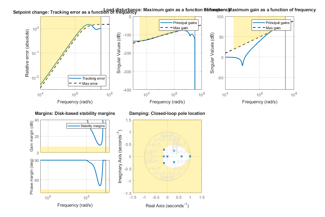
The best design satisfies the hard constraints (Hard less than 1) and nearly satisfies the other constraints (Soft close to 1). Verify this graphically by plotting the tuned responses for each requirement.
figure('Position',[10,10,1071,714])
viewGoal([Req1 Req2 Req3 Req4 Req5],ST)
Validation
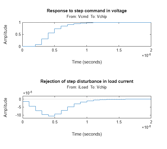
First validate the design in the linear domain using the slTuner interface. Plot the closed-loop response to a step command Vcmd and a step disturbance iLoad.
figure('Position',[100,100,560,500])
subplot(2,1,1)
step(getIOTransfer(ST,'Vcmd','Vchip'),20*Tm)
title('Response to step command in voltage')
subplot(2,1,2)
step(getIOTransfer(ST,'iLoad','Vchip'),20*Tm)
title('Rejection of step disturbance in load current')
Use getLoopTransfer to compute the open-loop response at the plant input and superimpose the plant and feedback compensator responses.
clf
L = getLoopTransfer(ST,'Vin',-1);
C = getBlockValue(ST,'compensator');
bodeplot(L,psmodel(2),C(2),{1e-3/Tm pi/Tm})
grid
legend('Open-loop response','Plant','Compensator')
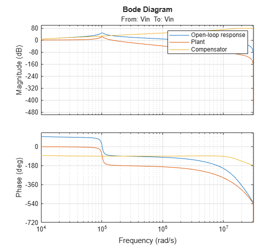
The controller achieves the desired bandwidth and the responses are fast enough. Apply the tuned parameter values to the Simulink model and simulate the tuned responses.
writeBlockValue(ST)
The results from the nonlinear simulation appear below. Note that the control signal Vin remains approximately within  saturation bounds for the setpoint tracking portion of the simulation.
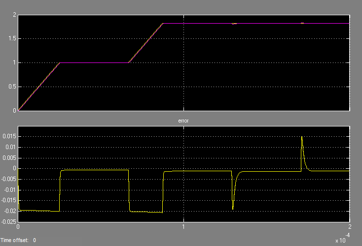
Figure 1: Response to ramp command and step load disturbances.

Figure 2: Amplitude of input voltage Vin during setpoint tracking phase.
See Also
systune (slTuner) | slTuner | TuningGoal.Tracking | TuningGoal.Gain | TuningGoal.Margins