Stability Margins in Control System Tuning
In control system tuning, you specify target gain and phase margins using Margins Goal (for Control System Tuner) or TuningGoal.Margins (for systune). The software provides tools
to help you visualize and interpret the gain and phase margins in your tuned system.
Gain and Phase Margins
Gain and phase margins measure the tolerance of a control loop to variations in the
open-loop system response. The Margins Goal and TuningGoal.Margins rely on the notion of a disk margin
to compute gain and phase margins. Like classical gain and phase margins, disk margins
quantify the stability of a closed-loop system against gain or phase variations in the
open-loop response. Disk margins also take into account all frequencies and loop
interactions. Therefore, disk-based margin analysis provides a stronger guarantee of
stability than the classical gain and phase margins. For more information about disk
margins, see Stability Analysis Using Disk Margins (Robust Control Toolbox).
For a SISO system, the gain and phase margins indicate how much the gain or phase of the open-loop response L can change without loss of stability.
For MIMO systems, gain and phase margins are interpreted as follows:
Gain margin — Stability is preserved when the gain changes up to the gain margin value in each feedback channel. The gain can change in all channels simultaneously, and by a different amount in each channel.
Phase margin — Stability is preserved when the phase changes up to the phase margin value in each feedback channel. The phase can change in all channels simultaneously, and by a different amount in each channel.
Gain and phase margins typically vary across frequencies. For example, in a SISO loop, a gain margin of 5 dB at 2 rad/s indicates that closed-loop stability is maintained when the loop gain increases or decreases by as much as 5 dB at this frequency. For control system tuning, you specify target values for the minimum (worst) margins across all frequencies. The margin tuning goal assumes symmetric ranges of variation, such as ±5 dB or ±30°.
Interpret Gain and Phase Margin Plots
For control system tuning, visualize system stability margins to help evaluate the performance of the tuned system.
In Control System Tuner, use a Margins Goal or Quick Loop Tuning.
At the command line, use
viewGoal. For instance, ifSis the control system, andReqis aTuningGoal.Marginsgoal, enter the following.viewGoal(Req,S)
viewGoal produces a plot with a yellow shaded region where the
target margins are not met. The plot also shows the gain and phase margins for the current
values of the tunable parameters in the control system. These margins appear as a blue trace
that typically varies across frequencies. For instance, the following plot shows a typical
result.
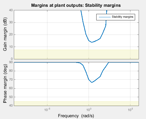
The plot shows that the frequency of the gain or phase variation can affect how large a perturbation the system can tolerate without going unstable. The minimum (worst) gain and phase margins occur at about 2 rad/s. At this frequency, the system can tolerate changes in open-loop gain of about ±14 dB, or changes in phase of about ±66°. For this system, the margins at all frequencies are well above the target margins used for tuning, shown in yellow.
Simultaneous Gain and Phase Variations
In general, gain margins are determined assuming no phase variation, and phase margins
are determined assuming no gain variation. In practice, your system can experience
simultaneous gain and phase variations. Disk-based margin analysis also gives you a range of
simultaneous gain and phase variations that the system can tolerate. For instance, suppose
that your system has a disk-based gain margin of 5 dB. This system remains stable for gain
changes of ±5 dB, assuming no phase variation. Use the diskmarginplot (Robust Control Toolbox)
command to visualize the region of simultaneous gain and phase variations that the system
can tolerate.
diskmarginplot(db2mag(5))
![Plot of simultaneous gain and phase variation for a system with disk-based gain margin DGM = [0.56,1.8] and disk-based phase margin DPM = 31°.](margins_robustness.png)
The shaded region shows the stable range of combined gain and phase variations for a
disk-based gain margin of 5 dB. With no phase variation, the system can tolerate the full
range of gain variation, –5 dB to 5 dB, or gain that changes by a factor within the range
DGM = [0.56,1.8]. Adding in phase variation reduces the tolerable gain
variation. For instance, If the phase is allowed to vary by ±25°, the tolerable gain
variation drops to a range of about ±3 dB. The disk-based phase margin is the allowable
phase variation when there is no gain variation, in this case about ±31°, shown in the plot
as DPM.
For more information about disk margins, see Stability Analysis Using Disk Margins (Robust Control Toolbox).
Algorithm
The gain and phase margin values are both derived from the disk margin. The disk margin measures the radius of a circular exclusion region centered near the critical point. (See Stability Analysis Using Disk Margins (Robust Control Toolbox).) For a system with open-loop response L(jω), this radius ɑ is a function of the scaled norm:
Unlike classical gain and phase margins, the disk margins and associated gain and phase margins guarantee that the open-loop response stays at a safe distance from the critical point at all frequencies.
Impact of Scaling
The frequency dependence of the gain and phase margins can be obtained by an exact calculation involving μ-analysis. However, for computational efficiency, the tuning algorithm uses an approximate calculation with a constant scaling D instead of the frequency-dependent scaling D(jω):
This approximation is an upper bound on 1/ɑ, or a lower bound on ɑ. It can therefore yield smaller margins in parts of the frequency range, especially at frequencies away from the frequency at which the minimum margin occurs. The smaller margin is still a guaranteed margin, but it might be more conservative than the true margin. To see the lower bound used by the tuning algorithm, right-click on the stability-margins plot and select Systems > Tuned lower bound.
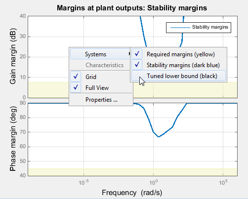
If you see a significant gap between the actual margins of the tuned system (blue
curve) and the lower-bound approximation used for tuning (black curve), try increasing the
D-scaling order to introduce some frequency dependence into the scaling. For tuning in
Control System Tuner, set the D-scaling order in the Margins Goal dialog box.
For command-line tuning, set this value using the ScalingOrder property
of TuningGoal.Margins. The default order is zero
(static scaling).
See Also
TuningGoal.Margins | diskmargin (Robust Control Toolbox) | viewGoal
Topics
- Loop Shape and Stability Margin Specifications
- Margins Goal
- Stability Analysis Using Disk Margins (Robust Control Toolbox)