Multiloop Control of a Helicopter
This example shows how to use slTuner and systune to tune a multiloop controller for a rotorcraft.
Helicopter Model
This example uses an 8-state helicopter model at the hovering trim condition. The state vector x = [u,w,q,theta,v,p,phi,r] consists of
Longitudinal velocity
u(m/s)Lateral velocity
v(m/s)Normal velocity
w(m/s)Pitch angle
theta(deg)Roll angle
phi(deg)Roll rate
p(deg/s)Pitch rate
q(deg/s)Yaw rate
r(deg/s).
The controller generates commands ds,dc,dT in degrees for the longitudinal cyclic, lateral cyclic, and tail rotor collective using measurements of theta, phi, p, q, and r.
Control Architecture
The following Simulink® model depicts the control architecture:
open_system('rct_helico')
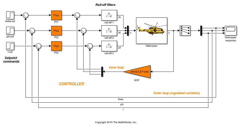
The control system consists of two feedback loops. The inner loop (static output feedback) provides stability augmentation and decoupling. The outer loop (PI controllers) provides the desired setpoint tracking performance. The main control objectives are as follows:
Track setpoint changes in
theta,phi, andrwith zero steady-state error, rise times of about 2 seconds, minimal overshoot, and minimal cross-couplingLimit the control bandwidth to guard against neglected high-frequency rotor dynamics and measurement noise
Provide strong multivariable gain and phase margins (robustness to simultaneous gain/phase variations at the plant inputs and outputs, see
diskmarginfor details).
We use lowpass filters with cutoff at 40 rad/s to partially enforce the second objective.
Controller Tuning
You can jointly tune the inner and outer loops with the systune command. This command only requires models of the plant and controller along with the desired bandwidth (which is a function of the desired response time). When the control system is modeled in Simulink, you can use the slTuner interface to quickly set up the tuning task. Create an instance of this interface with the list of blocks to be tuned.
ST0 = slTuner('rct_helico',{'PI1','PI2','PI3','SOF'});
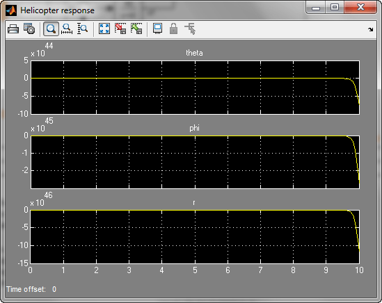
Each tunable block is automatically parameterized according to its type and initialized with its value in the Simulink model ( for the PI controllers and zero for the static output-feedback gain). Simulating the model shows that the control system is unstable for these initial values:
Mark the I/O signals of interest for setpoint tracking, and identify the plant inputs and outputs (control and measurement signals) where the stability margin are measured.
addPoint(ST0,{'theta-ref','phi-ref','r-ref'})   % setpoint commands
addPoint(ST0,{'theta','phi','r'})               % corresponding outputs
addPoint(ST0,{'u','y'});
Finally, capture the design requirements using TuningGoal objects. We use the following requirements for this example:
Tracking requirement: The response of
theta,phi,rto step commandstheta_ref,phi_ref,r_refmust resemble a decoupled first-order response with a one-second time constantStability margins: The multivariable gain and phase margins at the plant inputs
uand plant outputsymust be at least 5 dB and 40 degreesFast dynamics: The magnitude of the closed-loop poles must not exceed 25 to prevent fast dynamics and jerky transients
% Less than 20% mismatch with reference model 1/(s+1)
TrackReq = TuningGoal.StepTracking({'theta-ref','phi-ref','r-ref'},{'theta','phi','r'},1);
TrackReq.RelGap = 0.2;

% Gain and phase margins at plant inputs and outputs
MarginReq1 = TuningGoal.Margins('u',5,40);
MarginReq2 = TuningGoal.Margins('y',5,40);

% Limit on fast dynamics
MaxFrequency = 25;
PoleReq = TuningGoal.Poles(0,0,MaxFrequency);
You can now use systune to jointly tune all controller parameters. This returns the tuned version ST1 of the control system ST0.
AllReqs = [TrackReq,MarginReq1,MarginReq2,PoleReq];
ST1 = systune(ST0,AllReqs);
Final: Soft = 1.12, Hard = -Inf, Iterations = 72
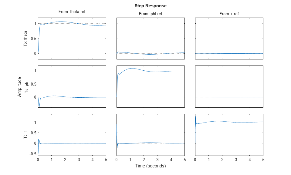
The final value is close to 1 so the requirements are nearly met. Plot the tuned responses to step commands in theta, phi, r:
T1 = getIOTransfer(ST1,{'theta-ref','phi-ref','r-ref'},{'theta','phi','r'});
step(T1,5)
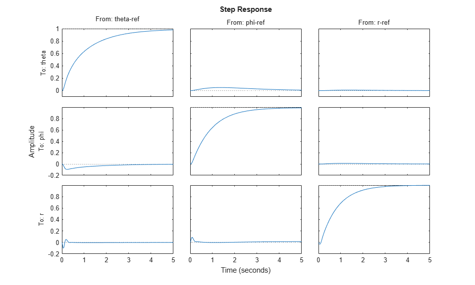
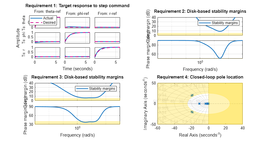
The rise time is about two seconds with no overshoot and little cross-coupling. You can use viewGoal for a more thorough validation of each requirement, including a visual assessment of the multivariable stability margins (see diskmargin for details):
figure('Position',[100,100,900,474])
viewGoal(AllReqs,ST1)
Inspect the tuned values of the PI controllers and static output-feedback gain.
showTunable(ST1)
Block 1: rct_helico/PI1 =

             1
  Kp + Ki * ---
             s

  with Kp = 1.04, Ki = 2.08

Name: PI1
Continuous-time PI controller in parallel form.

-----------------------------------

Block 2: rct_helico/PI2 =

             1
  Kp + Ki * ---
             s

  with Kp = -0.0938, Ki = -1.35

Name: PI2
Continuous-time PI controller in parallel form.

-----------------------------------

Block 3: rct_helico/PI3 =

             1
  Kp + Ki * ---
             s

  with Kp = 0.135, Ki = -2.2

Name: PI3
Continuous-time PI controller in parallel form.

-----------------------------------

Block 4: rct_helico/SOF =

  D =
              u1         u2         u3         u4         u5
   y1      2.222    -0.3115  -0.003376     0.7858   -0.01526
   y2    -0.1904     -1.284    0.01846   -0.08301    -0.1189
   y3   -0.02352   -0.02127     -1.893  -0.002861    0.06788

Name: SOF
Static gain.
Benefit of the Inner Loop
You may wonder whether the static output feedback is necessary and whether PID controllers aren't enough to control the helicopter. This question is easily answered by re-tuning the controller with the inner loop open. First break the inner loop by adding a loop opening after the SOF block:
addOpening(ST0,'SOF')
Then remove the SOF block from the tunable block list and re-parameterize the PI blocks as full-blown PIDs with the correct loop signs (as inferred from the first design).
PID = pid(0,0.001,0.001,.01);  % initial guess for PID controllers

removeBlock(ST0,'SOF');
setBlockParam(ST0,...
   'PI1',tunablePID('C1',PID),...
   'PI2',tunablePID('C2',-PID),...
   'PI3',tunablePID('C3',-PID));
Re-tune the three PID controllers and plot the closed-loop step responses.
ST2 = systune(ST0,AllReqs);
Final: Soft = 4.94, Hard = -Inf, Iterations = 67
T2 = getIOTransfer(ST2,{'theta-ref','phi-ref','r-ref'},{'theta','phi','r'});
figure, step(T2,5)
The final value is no longer close to 1 and the step responses confirm the poorer performance with regard to rise time, overshoot, and decoupling. This suggests that the inner loop has an important stabilizing effect that should be preserved.
See Also
systune (slTuner) | slTuner | TuningGoal.StepTracking | TuningGoal.Margins | TuningGoal.Poles