Validating Results
This example shows how to interpret and validate tuning results from systune.
Background
You can tune the parameters of your control system with systune or looptune. The design specifications are captured using TuningGoal requirement objects. This example shows how to interpret the results from systune, graphically verify the design requirements, and perform additional open- and closed-loop analysis.
Controller Tuning with SYSTUNE
We use an autopilot tuning application as illustration; see the "Tuning of a Two-Loop Autopilot" example for details. The tuned compensator is the "MIMO Controller" block highlighted in orange in the model below.
open_system('rct_airframe2')

The setup and tuning steps are repeated below for completeness.
ST0 = slTuner('rct_airframe2','MIMO Controller');

% Compensator parameterization
C0 = tunableSS('C',2,1,2);
C0.D.Value(1) = 0;
C0.D.Free(1) = false;
setBlockParam(ST0,'MIMO Controller',C0)

% Requirements
Req1 = TuningGoal.Tracking('az ref','az',1);                  % tracking
Req2 = TuningGoal.Gain('delta fin','delta fin',tf(25,[1 0])); % roll-off
Req3 = TuningGoal.Margins('delta fin',7,45);                  % margins
MaxGain = frd([2 200 200],[0.02 2 200]);
Req4 = TuningGoal.Gain('delta fin','az',MaxGain);  % disturbance rejection

% Tuning
Opt = systuneOptions('RandomStart',3);
rng('default')
[ST1,fSoft] = systune(ST0,[Req1,Req2,Req3,Req4],Opt);
Final: Soft = 1.51, Hard = -Inf, Iterations = 52
Final: Soft = 1.15, Hard = -Inf, Iterations = 125
Final: Soft = 1.15, Hard = -Inf, Iterations = 72
Final: Soft = 1.15, Hard = -Inf, Iterations = 109
Interpreting Results
systune run three optimizations from three different starting points and returned the best overall result. The first output ST is an slTuner interface representing the tuned control system. The second output fSoft contains the final values of the four requirements for the best design.
fSoft
fSoft =

    1.1476    1.1476    0.5461    1.1476
Requirements are normalized so a requirement is satisfied if and only if its value is less than 1. Inspection of fSoft reveals that Requirements 1,2,4 are active and slightly violated while Requirement 3 (stability margins) is satisfied.
Verifying Requirements
Use viewGoal to graphically inspect each requirement. This is useful to understand whether small violations are acceptable or what causes large violations. First verify the tracking requirement.
viewGoal(Req1,ST1)
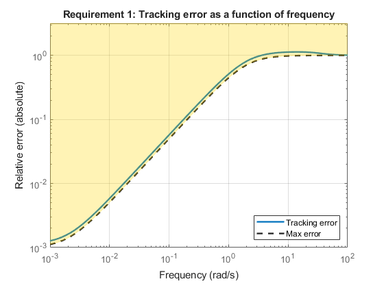
We observe a slight violation across frequency, suggesting that setpoint tracking will perform close to expectations. Similarly, verify the disturbance rejection requirement.
viewGoal(Req4,ST1)
legend('location','NorthWest')
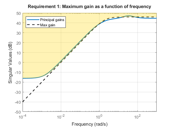
Most of the violation is at low frequency with a small bump near 35 rad/s, suggesting possible damped oscillations at this frequency. Finally, verify the stability margin requirement.
viewGoal(Req3,ST1)

This requirement is satisfied at all frequencies, with the smallest margins achieved near the crossover frequency as expected.
Evaluating Requirements
You can also use evalGoal to evaluate each requirement, that is, compute its contribution to the soft and hard constraints. For example
[H1,f1] = evalGoal(Req1,ST1);
returns the value f1 of the requirement and the underlying frequency-weighted transfer function H1 used to computed it. You can verify that f1 matches the first entry of fSoft and coincides with the peak gain of H1.
[f1 fSoft(1) getPeakGain(H1,1e-6)]
ans =

    1.1476    1.1476    1.1476
Analyzing System Responses
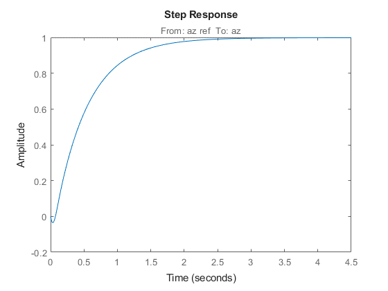
In addition to verifying requirements, you can perform basic open- and closed-loop analysis using getIOTransfer and getLoopTransfer. For example, verify tracking performance in the time domain by plotting the response az to a step command azref for the tuned system ST1.
T = ST1.getIOTransfer('az ref','az');
step(T)
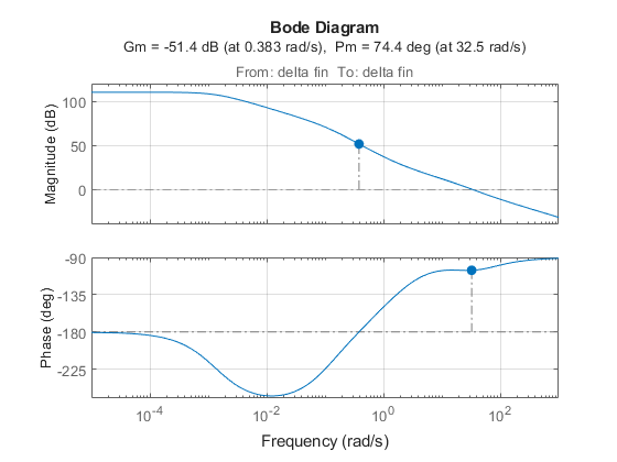
Also plot the open-loop response measured at the plant input delta fin. You can use this plot to assess the classical gain and phase margins at the plant input.
L = ST1.getLoopTransfer('delta fin',-1);  % negative-feedback loop transfer
margin(L)
grid
Soft vs Hard Requirements
So far we have treated all four requirements equally in the objective function. Alternatively, you can use a mix of soft and hard constraints to differentiate between must-have and nice-to-have requirements. For example, you could treat Requirements 3,4 as hard constraints and optimize the first two requirements subject to these constraints. For best results, do this only after obtaining a reasonable design with all requirements treated equally.
[ST2,fSoft,gHard] = systune(ST1,[Req1 Req2],[Req3 Req4]);
Final: Soft = 1.29, Hard = 0.99973, Iterations = 101
fSoft
fSoft =

    1.2889    1.2894
gHard
gHard =

    0.4665    0.9997
Here fSoft contains the final values of the first two requirements (soft constraints) and gHard contains the final values of the last two requirements (hard constraints). The hard constraints are satisfied since all entries of gHard are less than 1. As expected, the best value of the first two requirements went up as the optimizer strived to strictly enforce the fourth requirement.