Estimate Model Parameters and Initial States (GUI)
This example shows how to estimate the physical parameters - mass (m), spring constant (k), and damping (b) of a simple mass-spring-damper model. This example illustrates the significance of initial state estimation.
Mass Spring Damper System Model
Open the Simulink® model.
open_system("msd_system")

The model output is the displacement response (position) of the mass in a mass-spring-damper system, subject to a constant force (F), and an initial displacement (x0). x0 is the initial condition of the Position integrator block. Run the simulation once to observe the response of the model to a nominal set of parameter values.
Experimental Data Sets
For estimation of the model parameters (m, b, and k), two sets of experimental data are used. These data sets were obtained using two different initial positions (0.1 and 0.3), and contain additive noise. Following is the plot of these data sets, along with the simulated response, pos, of the Simulink model for x0=–0.1 and a nominal set of parameter values (m=8, k=500, b=100).

Estimation of Model Parameters
The model has three parameters (k, b, m) that appear in the Gain blocks of the Simulink model msd_system. We estimate these parameters using Parameter Estimation.
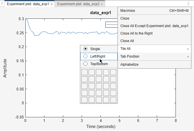
Double-click the Parameter Estimation GUI with preloaded data block in the model to open a pre-configured estimation GUI session. The experimental data sets are already loaded in the project (data_exp1 and data_exp2). To lay out the plots so that the Experiment plot:data_exp1 and Experiment plot:data_exp2 plots are both visible, click the Document actions button. In the dropdown menu, click Tile All > Left/Right.
Click Plot Model Response to simulate the model for the two experiments. The plots show that the model simulation does not match the experiment data.

Parameter Estimation with No State Estimation
The app is configured to estimate the model parameters using both data_exp1 and data_exp2 experiments; click Select Parameters to see the selected parameters and Select Experiments to see the experiments selected for estimation.
Click Estimate to start the estimation. You can modify estimation options by setting the Cost Function combobox and clicking More Options.
While the estimation is running, the plots update and a dialog box showing estimation progress appears. The progress dialog box shows the estimation iterations, the number of times the model has been evaluated (F-count), and the estimation cost at each iteration.


After a number of iterations the estimation converges and terminates. The model is updated with the estimated parameters and the estimation results are saved in the data browser.
The data_exp1 and data_exp2 experiment plots show that the model parameters have been tuned to match the measured experiment data as closely as possible. The simulated measured signals match well from the 2 second mark onward but don't match well before 2 seconds. The simulation results for both experiments start at –0.1. This is the initial condition of the model which was not estimated; these plots show that the initial condition should also be estimated.
Parameter Estimation with Initial State Estimation
The data_exp1 and data_exp2 experiments specify the measured output data but as seen above must also specify the model initial state. Add the initial states to the experiments and estimate them.
Right-click data_exp1 and select Edit to open a dialog box to configure the experiment.

Click Select Initial States and select the position state. Click OK to close the state selector and add the selected state to the experiment.


Right-click data_exp2 and select Edit and add the position state to the experiment.
The experiments are now configured to include initial states that can be estimated. Click Select Parameters.

The upper portion of the select parameters dialog box has a section for parameters that are tuned using all experiments selected for estimation. The lower section of the dialog box has a combo-box to select an experiment and widgets to specify initial states and parameters that are tuned using only the selected experiment. For this problem, the data_exp1 and data_exp2 experiments estimate the model initial state for each experiment.
You can now start the estimation, but first create plots to monitor the estimation progress. Click Add Plot and select Parameter Trajectory, right click the plot and select Show scaled values. This creates a plot that shows how the estimated parameter values change during estimation. To lay out the plots so that the Experiment plot:data_exp1, Experiment plot:data_exp2, and EstimatedParams plots are all visible, drag the plot tabs or use the Document actions button.
Click the Estimate button to start the estimation.

After a number of iterations the estimation converges and terminates. The data_exp1 and data_exp2 experiment plots show how estimating the initial value improves the estimation fit. The EstimatedParams plot shows the estimated initial state for the two experiments, the plot also shows that the estimated k value did not change while b and m changed slightly. You can confirm this by clicking EstimatedParams and examining the preview pane and then clicking EstimatedParams1 and examining the preview pane. Alternatively right click EstimatedParams and select Open to open a dialog box to view the results.

This example shows that it is important to independently estimate initial states for each experiment in order to obtain the correct estimates of the model parameters.
Related Examples
To learn how to estimate model parameters and initial states using the sdo.optimize command, see Estimate Model Parameters and Initial States (Code).