Saturable Transformer

Implement two- or three-winding saturable transformer

Library

Simscape / Electrical / Specialized Power Systems / Power Grid Elements

• 

Description

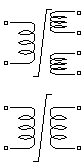
The Saturable Transformer block model shown consists of three coupled windings wound on the same core.

The model takes into account the winding resistances (R1 R2 R3) and the leakage inductances (L1 L2 L3) as well as the magnetizing characteristics of the core, which is modeled by a resistance Rm simulating the core active losses and a saturable inductance Lsat.

You can choose one of the following two options for the modeling of the nonlinear flux-current characteristic

1. Model saturation without hysteresis. The total iron losses (eddy current + hysteresis) are modeled by a linear resistance, Rm.

2. Model hysteresis and saturation. Specification of the hysteresis is done by means of the Hysteresis Design Tool of the Powergui block. The eddy current losses in the core are modeled by a linear resistance, Rm.

   Note

   Modeling the hysteresis requires additional computation load and therefore slows down the simulation. The hysteresis model should be reserved for specific applications where this phenomenon is important.

Saturation Characteristic Without Hysteresis

When the hysteresis is not modeled, the saturation characteristic of the Saturable Transformer block is defined by a piecewise linear relationship between the flux and the magnetization current.

Therefore, if you want to specify a residual flux, phi0, the second point of the saturation characteristic should correspond to a null current, as shown in the figure (b).

The saturation characteristic is entered as (i, phi) pair values in per units, starting with pair (0, 0). The software converts the vector of fluxes Φpu and the vector of currents Ipu into standard units to be used in the saturation model of the Saturable Transformer block:

Φ = Φ_puΦ_baseI = I_puI_base,

where the base flux linkage (Φ_base) and base current (I_base) are the peak values obtained at nominal voltage power and frequency:

$$\begin{array}{c}{I}_{\text{base}}=\frac{Pn}{V_1}\sqrt{2}\\ {\Phi }_{\text{base}}=\frac{V_1}{2\pi f_n}\sqrt{2}.\end{array}$$

The base flux is defined as the peak value of the sinusoidal flux (in webers) when winding 1 is connected to a 1 pu sinusoidal voltage source (nominal voltage). The Φ_base value defined above represents the base flux linkage (in volt-seconds). It is related to the base flux by the following equation:

Φ_base = Base flux × number of turns of winding 1.

When they are expressed in pu, the flux and the flux linkage have the same value.

Saturation Characteristic with Hysteresis

The magnetizing current I is computed from the flux Φ obtained by integrating voltage across the magnetizing branch. The static model of hysteresis defines the relation between flux and the magnetization current evaluated in DC, when the eddy current losses are not present.

The hysteresis model is based on a semi-empirical characteristic, using an arctangent analytical expression Φ(I) and its inverse I(Φ) to represent the operating point trajectories. The analytical expression parameters are obtained by curve fitting empirical data defining the major loop and the single-valued saturation characteristic. The Hysteresis design tool of the Powergui block is used to fit the hysteresis major loop of a particular core type to basic parameters. These parameters are defined by the remanent flux (Φr), the coercive current (Ic), and the slope (dΦ/dI) at (0, Ic) point as shown in the next figure.

The major loop half cycle is defined by a series of N equidistant points connected by line segments. The value of N is defined in the Hysteresis design tool of the Powergui block. Using N = 256 yields a smooth curve and usually gives satisfactory results.

The single-valued saturation characteristic is defined by a set of current-flux pairs defining a saturation curve which should be asymptotic to the air core inductance Ls.

The main characteristics of the hysteresis model are summarized below:

1. A symmetrical variation of the flux produces a symmetrical current variation between -Imax and +Imax, resulting in a symmetrical hysteresis loop whose shape and area depend on the value of Φmax. The major loop is produced when Φmax is equal to the saturation flux (Φs). Beyond that point the characteristic reduces to a single-valued saturation characteristic.

2. In transient conditions, an oscillating magnetizing current produces minor asymmetrical loops, as shown in the next figure, and all points of operation are assumed to be within the major loop. Loops once closed have no more influence on the subsequent evolution.

   

The trajectory starts from the initial (or residual) flux point, which must lie on the vertical axis inside the major loop. You can specify this initial flux value phi0, or it is automatically adjusted so that the simulation starts in steady state.

The Per Unit Conversion

In order to comply with industry practice, the block allows you to specify the resistance and inductance of the windings in per unit (pu). The values are based on the transformer rated power Pn in VA, nominal frequency fn in Hz, and nominal voltage Vn, in Vrms, of the corresponding winding. For each winding the per unit resistance and inductance are defined as

$$\begin{array}{c}R(\text{p}\text{.u}\text{.})=\frac{R(\Omega )}{R_{\text{base}}}\\ L(\text{p}\text{.u}\text{.})=\frac{L(H)}{L_{\text{base}}}.\end{array}$$

The base resistance and base inductance used for each winding are

$$\begin{array}{c}{R}_{\text{base}}=\frac{V_n^2}{Pn}\\ L_{\text{base}}=\frac{R_{\text{base}}}{2\pi f_n}.\end{array}$$

For the magnetization resistance Rm, the pu values are based on the transformer rated power and on the nominal voltage of winding 1.

The default parameters of winding 1 specified in the dialog box section give the following base values:

$$\begin{array}{c}{R}_{\text{base}}=\frac{{\left(735\cdot {10}^3/\sqrt{3}\right)}^2}{250\cdot {10}^6}=720.3\Omega \\ L_{\text{base}}=\frac{720.3}{2\pi \cdot 60}=1.91H.\end{array}$$

For example, if winding 1 parameters are R1 = 1.44 Ω and L1 = 0.1528 H, the corresponding values to enter in the dialog box are

$$\begin{array}{c}{R}_1=\frac{1.44\Omega }{720.3\Omega }=0.002\text{ p}\text{.u}\text{.}\\ L_1=\frac{0.1528H}{1.91H}=0.08\text{ p}\text{.u}\text{.}\end{array}$$

Parameters

Configuration Tab

Three windings transformer

If selected, specify a saturable transformer with three windings; otherwise it implements a two windings transformer. Default is selected.

Simulate hysteresis

Select to model hysteresis saturation characteristic instead of a single-valued saturation curve. Default is cleared.

Hysteresis Mat file

The Hysteresis Mat file parameter is visible only if the Simulate hysteresis parameter is selected.

Specify a .mat file containing the data to be used for the hysteresis model. When you open the Hysteresis Design Tool of the Powergui, the default hysteresis loop and parameters saved in the hysteresis.mat file are displayed. Use the Load button of the Hysteresis Design tool to load another .mat file. Use the Save button of the Hysteresis Design tool to save your model in a new .mat file.

Measurements

Select Winding voltages to measure the voltage across the winding terminals of the Saturable Transformer block.

Select Winding currents to measure the current flowing through the windings of the Saturable Transformer block.

Select Flux and excitation current (Im + IRm) to measure the flux linkage, in volt seconds (V.s), and the total excitation current including iron losses modeled by Rm.

Select Flux and magnetization current (Im) to measure the flux linkage, in volt seconds (V.s), and the magnetization current, in amperes (A), not including iron losses modeled by Rm.

Select All measurement (V, I, Flux) to measure the winding voltages, currents, magnetization currents, and the flux linkage.

Default is None.

Place a Multimeter block in your model to display the selected measurements during the simulation.

In the Available Measurements list box of the Multimeter block, the measurements are identified by a label followed by the block name.

Measurement	Label
Winding voltages	Uw1:
Winding currents	Iw1:
Excitation current	Iexc:
Magnetization current	Imag:
Flux linkage	Flux:

Parameters Tab

Units

Specify the units used to enter the parameters of the Saturable Transformer block. Select pu to use per unit. Select SI to use SI units. Changing the Units parameter from pu to SI, or from SI to pu, will automatically convert the parameters displayed in the mask of the block. The per unit conversion is based on the transformer rated power Pn in VA, nominal frequency fn in Hz, and nominal voltage Vn, in Vrms, of the windings. Default is pu.

Nominal power and frequency

The nominal power rating, Pn, in volt-amperes (VA), and frequency, in hertz (Hz), of the transformer. Note that the nominal parameters have no impact on the transformer model when the Units parameter is set to SI. Default is [ 250e6 60 ].

Winding 1 parameters

The nominal voltage in volts RMS, resistance in pu or ohms, and leakage inductance in pu or Henrys for winding 1. Set the winding resistances and inductances to 0to implement an ideal winding. Default is [ 735e3 0.002 0.08 ] when the Units parameter is pu and [7.35e+05 4.3218 0.45856] when the Units parameter is SI .

Winding 2 parameters

The nominal voltage in volts RMS, resistance in pu or ohms, and leakage inductance in pu or Henrys for winding 2. Set the winding resistances and inductances to 0to implement an ideal winding. Default is [ 315e3 0.002 0.08 ] when the Units parameter is pu and [3.15e+05 0.7938 0.084225] when the Units parameter is SI.

Winding 3 parameters

The Winding 3 parameters are not available if the Three windings transformer parameter is not selected. The nominal voltage in volts RMS, resistance in pu or ohms, and leakage inductance in pu or Henrys for winding 3. Set the winding resistances and inductances to 0 to implement an ideal winding. Default is [ 315e3 0.002 0.08 ] when the Units parameter is pu and [3.15e+05 0.7938 0.084225] when the Units parameter is SI.

Saturation characteristic

Specify a series of magnetizing current (pu) - flux (pu) pairs starting with (0,0). Default is [ 0,0 ; 0.0024,1.2 ; 1.0,1.52 ] when the Units parameter is pu and [0 0;1.1545 3308.7;481.03 4191] when the Units parameter is SI.

Core loss resistance and initial flux

Specify the active power dissipated in the core by entering the equivalent resistance Rm in pu. For example, to specify a 0.2% of active power core loss at nominal voltage, use Rm = 500 pu. You can also specify the initial flux phi0 (pu). This initial flux becomes particularly important when the transformer is energized. If phi0 is not specified, the initial flux is automatically adjusted so that the simulation starts in steady state. When simulating hysteresis, Rm models the eddy current losses only. Default is [500] when the Units parameter is pu and 1.0805e+06 when the Units parameter is SI.

Advanced Tab

The Advanced tab of the block is not visible when you set the Simulation type parameter of the powergui block to Continuous, or when you select the Automatically handle discrete solver parameter of the powergui block. The tab is visible when you set the Simulation type parameter of the powergui block to Discrete, and when the Automatically handle discrete solver parameter of the powergui block is cleared.

Break Algebraic loop in discrete saturation model

When selected, a delay is inserted at the output of the saturation model computing magnetization current as a function of flux linkage (the integral of input voltage computed by a trapezoidal method). This delay eliminates the algebraic loop resulting from trapezoidal discretization methods and speeds up the simulation of the model. However, this delay introduces a one simulation step time delay in the model and can cause numerical oscillations if the sample time is too large. The algebraic loop is required in most cases to get an accurate solution.

When cleared (default), the discretization method of the saturation model is specified by the Discrete solver model parameter.

Discrete solver model

Select one of these methods to resolve the algebraic loop.

• Trapezoidal iterative—Although this method produces correct results, it is not recommended because Simulink^® tends to slow down and may fail to converge (simulation stops), especially when the number of saturable transformers is increased. Also, because of the Simulink algebraic loop constraint, this method cannot be used in real time. In R2018b and previous releases, you used this method when the Break Algebraic loop in discrete saturation model parameter was cleared.

• Trapezoidal robust—This method is slightly more accurate than the Backward Euler robust method. However, it may produce slightly damped numerical oscillations on transformer voltages when the transformer is at no load.

• Backward Euler robust—This method provides good accuracy and prevents oscillations when the transformer is at no load.

The maximum number of iterations for the robust methods is specified in the Preferences tab of the powergui block, in the Solver details for nonlinear elements section. For real time applications, you may need to limit the number of iterations. Usually, limiting the number of iterations to 2 produces acceptable results. The two robust solvers are the recommended methods for discretizing the saturation model of the transformer.

For more information on what method to use in your application, see Simulating Discretized Electrical Systems.

Limitations

Windings can be left floating (that is, not connected by an impedance to the rest of the circuit). However, the floating winding is connected internally to the main circuit through a resistor. This invisible connection does not affect voltage and current measurements.

Examples

The power_xfosaturable example illustrates the energization of one phase of a three-phase 450 MVA, 500/230 kV transformer on a 3000 MVA source. The transformer parameters are

Nominal power and frequency	Pn = 150e6 VA	fn = 60 Hz
Winding 1 parameters (primary)	V1 = 500e3 Vrms/sqrt(3)	R1 = 0.002 pu	L1 = 0.08 pu
Winding 2 parameters (secondary)	V2 = 230e3 Vrms/sqrt(3)	R2 = 0.002 pu	L2 = 0.08 pu
Saturation characteristic	[0 0; 0.0 1.2; 1.0 1.52]
Core loss resistance and initial flux	Rm = 500 pu	phi0 = 0.8 pu

Simulation of this circuit illustrates the saturation effect on the transformer current and voltage.

As the source is resonant at the fourth harmonic, you can observe a high fourth- harmonic content in the secondary voltage. In this circuit, the flux is calculated in two ways:

• By integrating the secondary voltage

• By using the Multimeter block

References

[1] Casoria, S., P. Brunelle, and G. Sybille, “Hysteresis Modeling in the MATLAB/Power System Blockset,” Electrimacs 2002, École de technologie supérieure, Montreal, 2002.

[2] Frame, J.G., N. Mohan, and Tsu-huei Liu, “Hysteresis modeling in an Electro-Magnetic Transients Program,” presented at the IEEE PES winter meeting, New York, January 31 to February 5, 1982.