kfoldMargin

Classification margins for cross-validated kernel ECOC model

Syntax

margin = kfoldMargin(CVMdl)

margin = kfoldMargin(CVMdl,Name,Value)

Description

margin = kfoldMargin(CVMdl) returns the classification margins obtained by the cross-validated kernel ECOC model (ClassificationPartitionedKernelECOC) CVMdl. For every fold, kfoldMargin computes the classification margins for validation-fold observations using a model trained on training-fold observations.

margin = kfoldMargin(CVMdl,Name,Value) returns classification margins with additional options specified by one or more name-value pair arguments. For example, specify the binary learner loss function, decoding scheme, or verbosity level.

Examples

Estimate k-Fold Cross-Validation Margins

Load Fisher's iris data set. X contains flower measurements, and Y contains the names of flower species.

load fisheriris
X = meas;
Y = species;

Cross-validate an ECOC model composed of kernel binary learners.

CVMdl = fitcecoc(X,Y,'Learners','kernel','CrossVal','on')

CVMdl = 
  ClassificationPartitionedKernelECOC
    CrossValidatedModel: 'KernelECOC'
           ResponseName: 'Y'
        NumObservations: 150
                  KFold: 10
              Partition: [1x1 cvpartition]
             ClassNames: {'setosa'  'versicolor'  'virginica'}
         ScoreTransform: 'none'

CVMdl is a ClassificationPartitionedKernelECOC model. By default, the software implements 10-fold cross-validation. To specify a different number of folds, use the 'KFold' name-value pair argument instead of 'Crossval'.

Estimate the classification margins for validation-fold observations.

m = kfoldMargin(CVMdl);
size(m)

ans = 1×2

   150     1

m is a 150-by-1 vector. m(j) is the classification margin for observation j.

Plot the k-fold margins using a boxplot.

boxplot(m,'Labels','All Observations')
title('Distribution of Margins')

Feature Selection Using k-Fold Margins

Perform feature selection by comparing k-fold margins from multiple models. Based solely on this criterion, the classifier with the greatest margins is the best classifier.

Load Fisher's iris data set. X contains flower measurements, and Y contains the names of flower species.

load fisheriris
X = meas;
Y = species;

Randomly choose half of the predictor variables.

rng(1); % For reproducibility
p = size(X,2); % Number of predictors
idxPart = randsample(p,ceil(0.5*p));

Cross-validate two ECOC models composed of kernel classification models: one that uses all of the predictors, and one that uses half of the predictors.

CVMdl = fitcecoc(X,Y,'Learners','kernel','CrossVal','on');
PCVMdl = fitcecoc(X(:,idxPart),Y,'Learners','kernel','CrossVal','on');

CVMdl and PCVMdl are ClassificationPartitionedKernelECOC models. By default, the software implements 10-fold cross-validation. To specify a different number of folds, use the 'KFold' name-value pair argument instead of 'Crossval'.

Estimate the k-fold margins for each classifier.

fullMargins = kfoldMargin(CVMdl);
partMargins = kfoldMargin(PCVMdl);

Plot the distribution of the margin sets using box plots.

boxplot([fullMargins partMargins], ...
    'Labels',{'All Predictors','Half of the Predictors'});
title('Distribution of Margins')

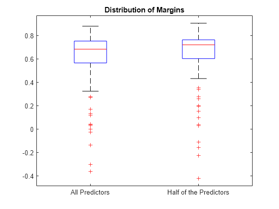
The PCVMdl margin distribution is similar to the CVMdl margin distribution.

Input Arguments

CVMdl — Cross-validated kernel ECOC model

ClassificationPartitionedKernelECOC model

Cross-validated kernel ECOC model, specified as a ClassificationPartitionedKernelECOC model. You can create a ClassificationPartitionedKernelECOC model by training an ECOC model using fitcecoc and specifying these name-value pair arguments:

• 'Learners'– Set the value to 'kernel', a template object returned by templateKernel, or a cell array of such template objects.

• One of the arguments 'CrossVal', 'CVPartition', 'Holdout', 'KFold', or 'Leaveout'.

Name-Value Arguments

Specify optional pairs of arguments as Name1=Value1,...,NameN=ValueN, where Name is the argument name and Value is the corresponding value. Name-value arguments must appear after other arguments, but the order of the pairs does not matter.

Before R2021a, use commas to separate each name and value, and enclose Name in quotes.

Example: kfoldMargin(CVMdl,'Verbose',1) specifies to display diagnostic messages in the Command Window.

BinaryLoss — Binary learner loss function

'hamming' | 'linear' | 'logit' | 'exponential' | 'binodeviance' | 'hinge' | 'quadratic' | function handle

Binary learner loss function, specified as the comma-separated pair consisting of 'BinaryLoss' and a built-in loss function name or function handle.

• This table contains names and descriptions of the built-in functions, where y_j is the class label for a particular binary learner (in the set {–1,1,0}), s_j is the score for observation j, and g(y_j,s_j) is the binary loss formula.

  Value	Description	Score Domain	g(yj,sj)
  'binodeviance'	Binomial deviance	(–∞,∞)	log[1 + exp(–2yjsj)]/[2log(2)]
  'exponential'	Exponential	(–∞,∞)	exp(–yjsj)/2
  'hamming'	Hamming	[0,1] or (–∞,∞)	[1 – sign(yjsj)]/2
  'hinge'	Hinge	(–∞,∞)	max(0,1 – yjsj)/2
  'linear'	Linear	(–∞,∞)	(1 – yjsj)/2
  'logit'	Logistic	(–∞,∞)	log[1 + exp(–yjsj)]/[2log(2)]
  'quadratic'	Quadratic	[0,1]	[1 – yj(2sj – 1)]2/2

  The software normalizes binary losses so that the loss is 0.5 when y_j = 0. Also, the software calculates the mean binary loss for each class [1].

• For a custom binary loss function, for example, customFunction, specify its function handle 'BinaryLoss',@customFunction.

  customFunction has this form:

  bLoss = customFunction(M,s)

  • M is the K-by-B coding matrix stored in Mdl.CodingMatrix.

  • s is the 1-by-B row vector of classification scores.

  • bLoss is the classification loss. This scalar aggregates the binary losses for every learner in a particular class. For example, you can use the mean binary loss to aggregate the loss over the learners for each class.

  • K is the number of classes.

  • B is the number of binary learners.

By default, if all binary learners are kernel classification models using SVM, then BinaryLoss is 'hinge'. If all binary learners are kernel classification models using logistic regression, then BinaryLoss is 'quadratic'.

Example: 'BinaryLoss','binodeviance'

Data Types: char | string | function_handle

Decoding — Decoding scheme

'lossweighted' (default) | 'lossbased'

Decoding scheme that aggregates the binary losses, specified as the comma-separated pair consisting of 'Decoding' and 'lossweighted' or 'lossbased'. For more information, see Binary Loss.

Example: 'Decoding','lossbased'

Options — Estimation options

[] (default) | structure array returned by statset

Estimation options, specified as the comma-separated pair consisting of 'Options' and a structure array returned by statset.

To invoke parallel computing:

• You need a Parallel Computing Toolbox™ license.

• Specify 'Options',statset('UseParallel',true).

Verbose — Verbosity level

0 (default) | 1

Verbosity level, specified as the comma-separated pair consisting of 'Verbose' and 0 or 1. Verbose controls the number of diagnostic messages that the software displays in the Command Window.

If Verbose is 0, then the software does not display diagnostic messages. Otherwise, the software displays diagnostic messages.

Example: 'Verbose',1

Data Types: single | double

Output Arguments

margin — Classification margins

numeric vector

Classification margins, returned as a numeric vector. margin is an n-by-1 vector, where each row is the margin of the corresponding observation and n is the number of observations (size(CVMdl.Y,1)).

More About

Classification Margin

The classification margin is, for each observation, the difference between the negative loss for the true class and the maximal negative loss among the false classes. If the margins are on the same scale, then they serve as a classification confidence measure. Among multiple classifiers, those that yield greater margins are better.

Binary Loss

The binary loss is a function of the class and classification score that determines how well a binary learner classifies an observation into the class. The decoding scheme of an ECOC model specifies how the software aggregates the binary losses and determines the predicted class for each observation.

Assume the following:

• m_kj is element (k,j) of the coding design matrix M—that is, the code corresponding to class k of binary learner j. M is a K-by-B matrix, where K is the number of classes, and B is the number of binary learners.

• s_j is the score of binary learner j for an observation.

• g is the binary loss function.

• $$\widehat{k}$$ is the predicted class for the observation.

The software supports two decoding schemes:

• Loss-based decoding [2] (Decoding is 'lossbased') — The predicted class of an observation corresponds to the class that produces the minimum average of the binary losses over all binary learners.

  $$\widehat{k}=\underset{k}{\text{argmin}}\frac{1}{B}{\displaystyle \sum _{j=1}^B\left|m_{kj}\right|g}(m_{kj},s_j).$$

• Loss-weighted decoding [3] (Decoding is 'lossweighted') — The predicted class of an observation corresponds to the class that produces the minimum average of the binary losses over the binary learners for the corresponding class.

  $$\widehat{k}=\underset{k}{\text{argmin}}\frac{{\displaystyle \sum _{j=1}^B\left|m_{kj}\right|g}(m_{kj},s_j)}{{\displaystyle \sum }_{j=1}^B\left|m_{kj}\right|}.$$

  The denominator corresponds to the number of binary learners for class k. [1] suggests that loss-weighted decoding improves classification accuracy by keeping loss values for all classes in the same dynamic range.

The predict, resubPredict, and kfoldPredict functions return the negated value of the objective function of argmin as the second output argument (NegLoss) for each observation and class.

This table summarizes the supported binary loss functions, where y_j is a class label for a particular binary learner (in the set {–1,1,0}), s_j is the score for observation j, and g(y_j,s_j) is the binary loss function.

Value	Description	Score Domain	g(yj,sj)
"binodeviance"	Binomial deviance	(–∞,∞)	log[1 + exp(–2yjsj)]/[2log(2)]
"exponential"	Exponential	(–∞,∞)	exp(–yjsj)/2
"hamming"	Hamming	[0,1] or (–∞,∞)	[1 – sign(yjsj)]/2
"hinge"	Hinge	(–∞,∞)	max(0,1 – yjsj)/2
"linear"	Linear	(–∞,∞)	(1 – yjsj)/2
"logit"	Logistic	(–∞,∞)	log[1 + exp(–yjsj)]/[2log(2)]
"quadratic"	Quadratic	[0,1]	[1 – yj(2sj – 1)]2/2

The software normalizes binary losses so that the loss is 0.5 when y_j = 0, and aggregates using the average of the binary learners [1].

Do not confuse the binary loss with the overall classification loss (specified by the LossFun name-value argument of the kfoldLoss and kfoldPredict object functions), which measures how well an ECOC classifier performs as a whole.

References

[1] Allwein, E., R. Schapire, and Y. Singer. “Reducing multiclass to binary: A unifying approach for margin classifiers.” Journal of Machine Learning Research. Vol. 1, 2000, pp. 113–141.

[2] Escalera, S., O. Pujol, and P. Radeva. “Separability of ternary codes for sparse designs of error-correcting output codes.” Pattern Recog. Lett. Vol. 30, Issue 3, 2009, pp. 285–297.

[3] Escalera, S., O. Pujol, and P. Radeva. “On the decoding process in ternary error-correcting output codes.” IEEE Transactions on Pattern Analysis and Machine Intelligence. Vol. 32, Issue 7, 2010, pp. 120–134.

Extended Capabilities

Automatic Parallel Support

Accelerate code by automatically running computation in parallel using Parallel Computing Toolbox™.

To run in parallel, specify the Options name-value argument in the call to this function and set the UseParallel field of the options structure to true using statset:

Options=statset(UseParallel=true)

For more information about parallel computing, see Run MATLAB Functions with Automatic Parallel Support (Parallel Computing Toolbox).

Version History

Introduced in R2018b

R2023b: Observations with missing predictor values are used in resubstitution and cross-validation computations

Starting in R2023b, the following classification model object functions use observations with missing predictor values as part of resubstitution ("resub") and cross-validation ("kfold") computations for classification edges, losses, margins, and predictions.

Model Type	Model Objects	Object Functions
Discriminant analysis classification model	ClassificationDiscriminant	resubEdge, resubLoss, resubMargin, resubPredict
	ClassificationPartitionedModel	kfoldEdge, kfoldLoss, kfoldMargin, kfoldPredict
Ensemble of discriminant analysis learners for classification	ClassificationEnsemble	resubEdge, resubLoss, resubMargin, resubPredict
	ClassificationPartitionedEnsemble	kfoldEdge, kfoldLoss, kfoldMargin, kfoldPredict
Gaussian kernel classification model	ClassificationPartitionedKernel	kfoldEdge, kfoldLoss, kfoldMargin, kfoldPredict
	ClassificationPartitionedKernelECOC	kfoldEdge, kfoldLoss, kfoldMargin, kfoldPredict
Linear classification model	ClassificationPartitionedLinear	kfoldEdge, kfoldLoss, kfoldMargin, kfoldPredict
	ClassificationPartitionedLinearECOC	kfoldEdge, kfoldLoss, kfoldMargin, kfoldPredict
Neural network classification model	ClassificationNeuralNetwork	resubEdge, resubLoss, resubMargin, resubPredict
	ClassificationPartitionedModel	kfoldEdge, kfoldLoss, kfoldMargin, kfoldPredict
Support vector machine (SVM) classification model	ClassificationSVM	resubEdge, resubLoss, resubMargin, resubPredict
	ClassificationPartitionedModel	kfoldEdge, kfoldLoss, kfoldMargin, kfoldPredict

In previous releases, the software omitted observations with missing predictor values from the resubstitution and cross-validation computations.