Markov Chain Analysis and Stationary Distribution

This example shows how to derive the symbolic stationary distribution of a trivial Markov chain by computing its eigen decomposition.

The stationary distribution represents the limiting, time-independent, distribution of the states for a Markov process as the number of steps or transitions increase.

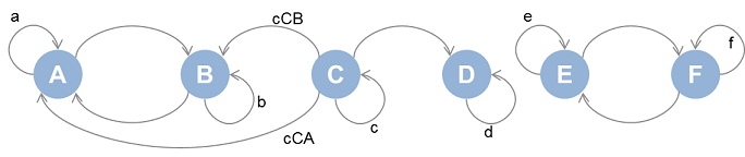
Define (positive) transition probabilities between states A through F as shown in the above image.

syms a b c d e f cCA cCB positive;

Add further assumptions bounding the transition probabilities. This will be helpful in selecting desirable stationary distributions later.

assumeAlso([a, b, c, e, f, cCA, cCB] < 1 & d == 1);

Define the transition matrix. States A through F are mapped to the columns and rows 1 through 6. Note the values in each row sum up to one.

P = sym(zeros(6,6));
P(1,1:2) = [a 1-a];
P(2,1:2) = [1-b b];
P(3,1:4) = [cCA cCB c (1-cCA-cCB-c)];
P(4,4) = d;
P(5,5:6) = [e 1-e];
P(6,5:6) = [1-f f];
P

P = 
$$\left(\begin{array}{cccccc}a& 1-a& 0& 0& 0& 0\\ 1-b& b& 0& 0& 0& 0\\ \mathrm{cCA}& \mathrm{cCB}& c& 1-\mathrm{cCA}-\mathrm{cCB}-c& 0& 0\\ 0& 0& 0& d& 0& 0\\ 0& 0& 0& 0& e& 1-e\\ 0& 0& 0& 0& 1-f& f\end{array}\right)$$

Compute all possible analytical stationary distributions of the states of the Markov chain. This is the problem of extracting eig with corresponding eigenvalues that can be equal to 1 for some value of the transition probabilities.

[V,D] = eig(P');

Analytical eigenvectors

V

V = 
$$\begin{array}{l}\left(\begin{array}{ccccccccc}\frac{b-1}{a-1}& 0& 0& -\frac{\left(c-d\right)\hspace{0.17em}\left(\mathrm{cCB}-b\hspace{0.17em}\mathrm{cCA}-b\hspace{0.17em}\mathrm{cCB}+c\hspace{0.17em}\mathrm{cCA}\right)}{{\sigma }_1}& \frac{b-1}{a-d}& 0& 0& -1& 0\\ 1& 0& 0& -\frac{\left(c-d\right)\hspace{0.17em}\left(\mathrm{cCA}-a\hspace{0.17em}\mathrm{cCA}-a\hspace{0.17em}\mathrm{cCB}+c\hspace{0.17em}\mathrm{cCB}\right)}{{\sigma }_1}& 1& 0& 0& 1& 0\\ 0& 0& 0& -\frac{c-d}{c+\mathrm{cCA}+\mathrm{cCB}-1}& 0& 0& 0& 0& 0\\ 0& 1& 0& 1& 0& 1& 0& 0& 0\\ 0& 0& \frac{f-1}{e-1}& 0& 0& 0& -\frac{f-1}{d-e}& 0& -1\\ 0& 1-d& 1& 0& 0& 0& 1& 0& 1\end{array}\right)\\ \\ \mathrm{where}\\ \\ \mathrm{ }{\sigma }_1=\left(c+\mathrm{cCA}+\mathrm{cCB}-1\right)\hspace{0.17em}\left(a+b-a\hspace{0.17em}c-b\hspace{0.17em}c+c^2-1\right)\end{array}$$

Analytical eigenvalues

diag(D)

ans = 
$$\left(\begin{array}{c}1\\ 1\\ c\\ d\\ a+b-1\\ e+f-1\end{array}\right)$$

Find eigenvalues that are exactly equal to 1. If there is any ambiguity in determining this condition for any eigenvalue, stop with an error - this way we are sure that below list of indices is reliable when this step is successful.

ix = find(isAlways(diag(D) == 1,'Unknown','error'));
diag(D(ix,ix))

ans = 
$$\left(\begin{array}{c}1\\ 1\\ d\end{array}\right)$$

Extract the analytical stationary distributions. The eigenvectors are normalized with the 1-norm or sum(abs(X)) prior to display.

for k = ix'
    V(:,k) = simplify(V(:,k)/norm(V(:,k)),1);
end
Probability = V(:,ix)

Probability = 
$$\begin{array}{l}\left(\begin{array}{ccc}\frac{b-1}{\left(a-1\right)\hspace{0.17em}{\sigma }_1}& 0& \frac{{\sigma }_5}{{\sigma }_2}\\ \frac{1}{{\sigma }_1}& 0& \frac{{\sigma }_6}{{\sigma }_2}\\ 0& 0& -\frac{c-1}{{\sigma }_3\hspace{0.17em}\left(c+\mathrm{cCA}+\mathrm{cCB}-1\right)}\\ 0& 1& \frac{1}{{\sigma }_3}\\ 0& 0& 0\\ 0& 0& 0\end{array}\right)\\ \\ \mathrm{where}\\ \\ \mathrm{ }{\sigma }_1=\sqrt{\frac{{\left(b-1\right)}^2}{{\left(a-1\right)}^2}+1}\\ \\ \mathrm{ }{\sigma }_2={\sigma }_3\hspace{0.17em}\left(c+\mathrm{cCA}+\mathrm{cCB}-1\right)\hspace{0.17em}\left(a+b-c-1\right)\\ \\ \mathrm{ }{\sigma }_3=\sqrt{\frac{{\left(c-1\right)}^2}{{\left(c+\mathrm{cCA}+\mathrm{cCB}-1\right)}^2}+\frac{{{\sigma }_6}^2}{{\sigma }_4}+\frac{{{\sigma }_5}^2}{{\sigma }_4}+1}\\ \\ \mathrm{ }{\sigma }_4={\left(c+\mathrm{cCA}+\mathrm{cCB}-1\right)}^2\hspace{0.17em}{\left(a+b-c-1\right)}^2\\ \\ \mathrm{ }{\sigma }_5=\mathrm{cCB}-b\hspace{0.17em}\mathrm{cCA}-b\hspace{0.17em}\mathrm{cCB}+c\hspace{0.17em}\mathrm{cCA}\\ \\ \mathrm{ }{\sigma }_6=\mathrm{cCA}-a\hspace{0.17em}\mathrm{cCA}-a\hspace{0.17em}\mathrm{cCB}+c\hspace{0.17em}\mathrm{cCB}\end{array}$$

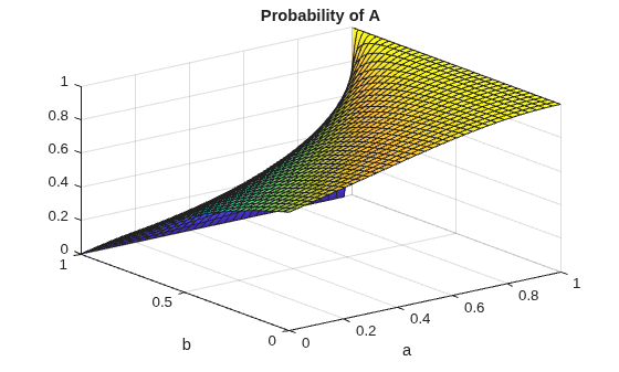
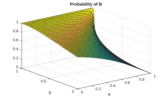
The probability of the steady state being A or B in the first eigenvector case is a function of the transition probabilities a and b. Visualize this dependency.

fsurf(Probability(1), [0 1 0 1]);
xlabel a
ylabel b
title('Probability of A');

figure(2);
fsurf(Probability(2), [0 1 0 1]);
xlabel a
ylabel b
title('Probability of B');

The stationary distributions confirm the following (Recall states A through F correspond to row indices 1 through 6 ):