Solve Differential Equations of RLC Circuit Using Laplace Transform

R2026b

Solve differential equations of an RLC circuit by using Laplace transforms in Symbolic Math Toolbox™ with this workflow. For simple examples on the Laplace transform, see laplace and ilaplace.

Definition: Laplace Transform

The Laplace transform of a function $f (t)$ is

$F (s) = \int_{0}^{\infty} f (t) e^{- ts} dt .$

Concept: Using Symbolic Workflows

Symbolic workflows keep calculations in the natural symbolic form instead of numeric form. This approach helps you understand the properties of your solution and use exact symbolic values. You substitute numbers in place of symbolic variables only when you require a numeric result or you cannot continue symbolically. For details, see Choose Numeric or Symbolic Arithmetic. Typically, the steps are:

Declare equations.
Solve equations.
Substitute values.
Plot results.
Analyze results.

Workflow: Solve RLC Circuit Using Laplace Transform

Declare Equations

You can use the Laplace transform to solve differential equations with initial conditions. For example, you can solve resistance-inductor-capacitor (RLC) circuits, such as this circuit.

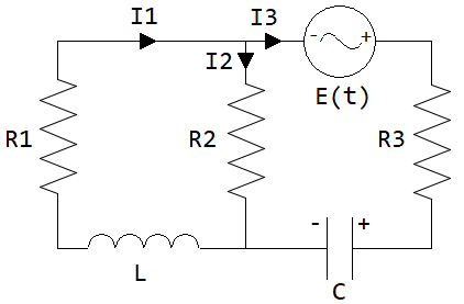
Resistances in ohm: $R_{1}, R_{2}, R_{3}$
Currents in ampere: $I_{1}, I_{2}, I_{3}$
Inductance in henry: $L$
Capacitance in farad: $C$
AC voltage source in volts: $E (t)$
Capacitor charge in coulomb: $Q (t)$

Apply Kirchhoff's voltage and current laws to get the following equations.

$\begin{array}{l} I_{1} = I_{2} + I_{3} \\ L \frac{{dI}_{1}}{dt} + I_{1} R_{1} + I_{2} R_{2} = 0 \\ E (t) + I_{2} R_{2} - \frac{Q}{C} - I_{3} R_{3} = 0 \end{array}$

Substitute the relation $I_{3} = d Q / d t$ (which is the rate of the capacitor being charged) to the above equations to get the differential equations for the RLC circuit.

$\begin{array}{l} \frac{{dI}_{1}}{dt} - \frac{R_{2}}{L} \frac{dQ}{dt} = - \frac{R_{1} + R_{2}}{L} I_{1} \\ \frac{dQ}{dt} = \frac{1}{R_{2} + R_{3}} (E (t) - \frac{Q}{C}) + \frac{R_{2}}{R_{2} + R_{3}} I_{1} \end{array}$

Declare the variables. Because the physical quantities have positive values, set the corresponding assumptions on the variables. Let $E (t)$ be an alternating voltage of 1 V.

syms L C I1(t) Q(t) s
R = sym('R%d',[1 3]);
assume([t L C R] > 0)
E(t) = 1*sin(t);        % AC voltage = 1 V

Declare the differential equations.

dI1 = diff(I1,t);
dQ = diff(Q,t);
eqn1 = dI1 - (R(2)/L)*dQ == -(R(1)+R(2))/L*I1

eqn1(t) = 
 $\frac{\partial}{\partial t} I_{1} (t) - \frac{R_{2} \frac{\partial}{\partial t} Q (t)}{L} = - \frac{I_{1} (t) (R_{1} + R_{2})}{L}$

eqn2 = dQ == (1/(R(2)+R(3))*(E-Q/C)) + R(2)/(R(2)+R(3))*I1

eqn2(t) = 
 $\frac{\partial}{\partial t} Q (t) = \frac{\sin (t) - \frac{Q (t)}{C}}{R_{2} + R_{3}} + \frac{R_{2} I_{1} (t)}{R_{2} + R_{3}}$

Solve Equations

Compute the Laplace transform of eqn1 and eqn2.

eqn1LT = laplace(eqn1,t,s)

eqn1LT = 
 $s laplace (I_{1} (t), t, s) - I_{1} (0) + \frac{R_{2} (Q (0) - s laplace (Q (t), t, s))}{L} = - \frac{(R_{1} + R_{2}) laplace (I_{1} (t), t, s)}{L}$

eqn2LT = laplace(eqn2,t,s)

eqn2LT = 
 $s laplace (Q (t), t, s) - Q (0) = \frac{R_{2} laplace (I_{1} (t), t, s)}{R_{2} + R_{3}} + \frac{\frac{C}{s^{2} + 1} - laplace (Q (t), t, s)}{C (R_{2} + R_{3})}$

The function solve solves only for symbolic variables. Therefore, to use solve, first substitute laplace(I1(t),t,s) and laplace(Q(t),t,s) with the variables I1_LT and Q_LT.

syms I1_LT Q_LT
eqn1LT = subs(eqn1LT,[laplace(I1,t,s) laplace(Q,t,s)],[I1_LT Q_LT])

eqn1LT = 
 $I_{1, LT} s - I_{1} (0) + \frac{R_{2} (Q (0) - Q_{LT} s)}{L} = - \frac{I_{1, LT} (R_{1} + R_{2})}{L}$

eqn2LT = subs(eqn2LT,[laplace(I1,t,s) laplace(Q,t,s)],[I1_LT Q_LT])

eqn2LT = 
 $Q_{LT} s - Q (0) = \frac{I_{1, LT} R_{2}}{R_{2} + R_{3}} - \frac{Q_{LT} - \frac{C}{s^{2} + 1}}{C (R_{2} + R_{3})}$

Solve the equations for I1_LT and Q_LT.

eqns = [eqn1LT eqn2LT];
vars = [I1_LT Q_LT];
[I1_LT, Q_LT] = solve(eqns,vars)

I1_LT = 
 $\frac{L I_{1} (0) - R_{2} Q (0) + C R_{2} s + L s^{2} I_{1} (0) - R_{2} s^{2} Q (0) + C L R_{2} s^{3} I_{1} (0) + C L R_{3} s^{3} I_{1} (0) + C L R_{2} s I_{1} (0) + C L R_{3} s I_{1} (0)}{(s^{2} + 1) (R_{1} + R_{2} + L s + C L R_{2} s^{2} + C L R_{3} s^{2} + C R_{1} R_{2} s + C R_{1} R_{3} s + C R_{2} R_{3} s)}$

Q_LT = 
 $\frac{C (R_{1} + R_{2} + L s + L R_{2} I_{1} (0) + R_{1} R_{2} Q (0) + R_{1} R_{3} Q (0) + R_{2} R_{3} Q (0) + L R_{2} s^{2} I_{1} (0) + L R_{2} s^{3} Q (0) + L R_{3} s^{3} Q (0) + R_{1} R_{2} s^{2} Q (0) + R_{1} R_{3} s^{2} Q (0) + R_{2} R_{3} s^{2} Q (0) + L R_{2} s Q (0) + L R_{3} s Q (0))}{(s^{2} + 1) (R_{1} + R_{2} + L s + C L R_{2} s^{2} + C L R_{3} s^{2} + C R_{1} R_{2} s + C R_{1} R_{3} s + C R_{2} R_{3} s)}$

Compute $I_{1}$ and $Q$ by computing the inverse Laplace transform of I1_LT and Q_LT. Simplify the result. Suppress the output because it is long.

I1sol = ilaplace(I1_LT,s,t);
Qsol = ilaplace(Q_LT,s,t);
I1sol = simplify(I1sol);
Qsol = simplify(Qsol);

Substitute Values

Before plotting the result, substitute symbolic variables by the numeric values of the circuit elements. Let $R_{1} = 4 Ω$ , $R_{2} = 2 Ω$ , $R_{3} = 3 Ω$ , $C = 1 / 4 F$ , $L = 1.6 H$ . Assume that the initial current is $I_{1} (0) = 2 A$ and the initial charge is $Q (0) = 2 C$ .

vars = [R L C I1(0) Q(0)];
values = [4 2 3 1.6 1/4 2 2];
I1sol = subs(I1sol,vars,values)

I1sol = 
 $\frac{200 \cos (t)}{8161} + \frac{405 \sin (t)}{8161} + \frac{16122 e^{- \frac{81 t}{40}} (\cosh (\frac{\sqrt{1761} t}{40}) - \frac{742529 \sqrt{1761} \sinh (\frac{\sqrt{1761} t}{40})}{14195421})}{8161}$

Qsol = subs(Qsol,vars,values)

Qsol = 
 $\frac{924 \sin (t)}{8161} - \frac{1055 \cos (t)}{8161} + \frac{17377 e^{- \frac{81 t}{40}} (\cosh (\frac{\sqrt{1761} t}{40}) + \frac{1109425 \sqrt{1761} \sinh (\frac{\sqrt{1761} t}{40})}{30600897})}{8161}$

Plot Results

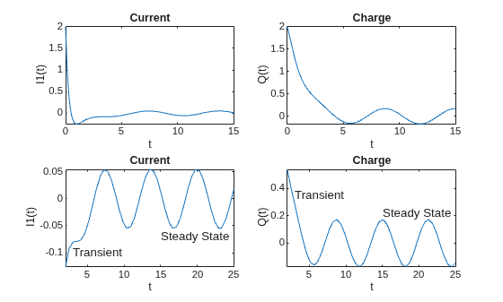
Plot the current I1sol and charge Qsol. Show both the transient and steady state behavior by using two different time intervals: $0 \leq t \leq 15$ and $2 \leq t \leq 25$ .

subplot(2,2,1)
fplot(I1sol,[0 15])                      
title('Current')
ylabel('I1(t)')
xlabel('t')

subplot(2,2,2)
fplot(Qsol,[0 15])                        
title('Charge')
ylabel('Q(t)')
xlabel('t')

subplot(2,2,3)
fplot(I1sol,[2 25])                  
title('Current')
ylabel('I1(t)')
xlabel('t')
text(3,-0.1,'Transient')
text(15,-0.07,'Steady State')

subplot(2,2,4)
fplot(Qsol,[2 25])                        
title('Charge')
ylabel('Q(t)')
xlabel('t')
text(3,0.35,'Transient')
text(15,0.22,'Steady State')

Analyze Results

Initially, the current and charge decrease exponentially. However, over the long term, they are oscillatory. These behaviors are called "transient" and "steady state", respectively. With the symbolic result, you can analyze the result's properties, which is not possible with numeric results.

Visually inspect I1sol and Qsol. They are a sum of terms. Find the terms by using children. Then, find the contributions of the terms by plotting them over [0 15]. The plots show the transient and steady state terms.

I1terms = children(I1sol);
I1terms = [I1terms{:}];
Qterms = children(Qsol);
Qterms = [Qterms{:}];

figure;
subplot(1,2,1)
fplot(I1terms,[0 15])
ylim([-0.5 2.5])
title('Current terms')

subplot(1,2,2)
fplot(Qterms,[0 15])
ylim([-0.5 2.5])
title('Charge terms')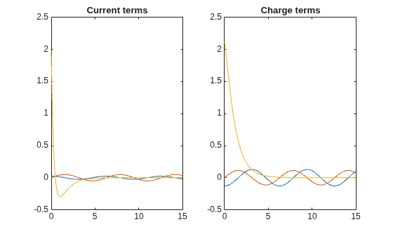

Figure contains 2 axes objects. Axes object 1 with title Current terms contains 3 objects of type functionline. Axes object 2 with title Charge terms contains 3 objects of type functionline.

The plots show that I1sol has a transient and steady state term, while Qsol has a transient and two steady state terms. From visual inspection, notice I1sol and Qsol have a term containing the exp function. Assume that this term causes the transient exponential decay. Separate the transient and steady state terms in I1sol and Qsol by checking terms for exp using has.

I1transient = I1terms(has(I1terms,'exp'))

I1transient = 
 $\frac{16122 e^{- \frac{81 t}{40}} (\cosh (\frac{\sqrt{1761} t}{40}) - \frac{742529 \sqrt{1761} \sinh (\frac{\sqrt{1761} t}{40})}{14195421})}{8161}$

I1steadystate = I1terms(~has(I1terms,'exp'))

I1steadystate = 
 $(\begin{array}{c} \frac{200 \cos (t)}{8161} & \frac{405 \sin (t)}{8161} \end{array})$

Similarly, separate Qsol into transient and steady state terms. This result demonstrates how symbolic calculations help you analyze your problem.

Qtransient = Qterms(has(Qterms,'exp'))

Qtransient = 
 $\frac{17377 e^{- \frac{81 t}{40}} (\cosh (\frac{\sqrt{1761} t}{40}) + \frac{1109425 \sqrt{1761} \sinh (\frac{\sqrt{1761} t}{40})}{30600897})}{8161}$

Qsteadystate = Qterms(~has(Qterms,'exp'))

Qsteadystate = 
 $(\begin{array}{c} - \frac{1055 \cos (t)}{8161} & \frac{924 \sin (t)}{8161} \end{array})$