Improve UAV Position Estimation with Kalman Filter

This example teaches you the basics of how to estimate the position of UAV by simulating a UAV that has a GPS sensor, and how to improve the position estimate by constructing a simple Kalman Filter.

Introduction to Position Estimation

To illustrate the importance of position estimation in autonomous navigation, imagine that you have arrived at a theme park, and you want to find your way to your favorite roller coaster, the CrazyCoaster2000, using a map like this:

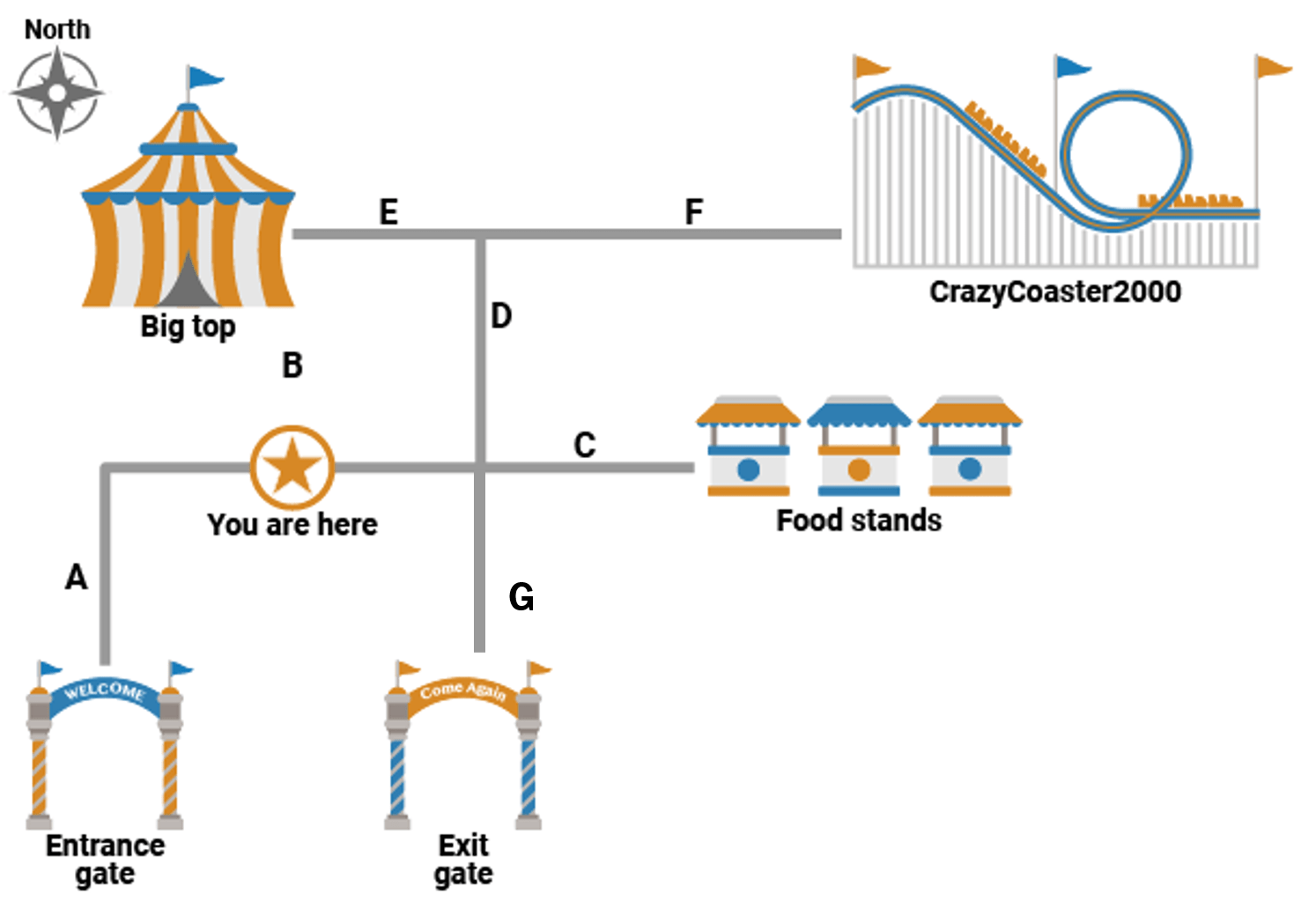
To use this map, you follow these steps:

1. Find out where you are in the map, as shown by the star.

2. Find out where the CrazyCoaster2000 is.

3. Determine the route to reach the coaster: go east on road B, north on road D, and east on road F.

As demonstrated, knowing your present position is the crucial first step of navigation, as your present position determines the route that you must take to reach your destination.

For a UAV performing autonomous navigation, the overall process is the same, where the UAV needs to know where it is at all times to make sure it is not lost. Typically, a UAV carries a GPS sensor to estimate its present location.

Simulate UAV with GPS Sensor

To illustrate the problem of relying on only GPS for position estimation, simulate a UAV that has a GPS sensor.

First, create a scenario with a stop time of 10 seconds, update rate of 10 Hz, and a reference location in Natick, Massachusetts.

localOrigin = [42.2825 -71.343 53.0352];
scenario = uavScenario(StopTime=10,UpdateRate=10,ReferenceLocation=localOrigin);

Create the trajectory for the UAV. Set the UAV to fly north for 10 meters at an altitude of 5 meters and a constant ground spees of 1 m/s.

targetWaypoint = [0  0 -5;
                 10 0 -5];
targetGroundSpeed = [1;1];
targetTrajectory = waypointTrajectory(targetWaypoint,GroundSpeed=targetGroundSpeed);

Create a UAV platform using the trajectory that you created

plat = uavPlatform("UAV",scenario,Trajectory=targetTrajectory);

Attach a GPS sensor with these properties to the UAV platform:

• UpdateRate of 10 Hz, which configures the GPS sensor to take 10 measurements per second.

• DecayFactor of 0.5, which gives the GPS a noise profile balanced between a white noise and random walk noise.

• Seed set to 10, which ensures the repeatability of the simulation.

• HorizontalPositionAccuracy and VerticalPositionAccuracy of 1.5 m, which sets the standard deviation of the noise in the horizontal and vertical position measurements.

gpsModel = gpsSensor(UpdateRate=10,DecayFactor=0.5, ...
    RandomStream="mt19937ar with seed",Seed=10,HorizontalPositionAccuracy=1.5, ...
    VerticalPositionAccuracy=1.5);
gps = uavSensor("GPS", plat, gpsModel);

Create structure arrays for storing the ground truth and GPS data.

groundTruthData = struct;
groundTruthData.Time = duration.empty;
groundTruthData.PositionX = zeros(0,1);
groundTruthData.PositionY = zeros(0,1);
groundTruthData.Altitude = zeros(0,1);

gpsData = struct;
gpsData.Time = duration.empty;
gpsData.PositionX = zeros(0,1);
gpsData.PositionY = zeros(0,1);
gpsData.Altitude = zeros(0,1);

Start the scenario.

setup(scenario)
updateCounter = 0;

while true
    % Advance scenario
    isRunning = advance(scenario);
    updateCounter = updateCounter + 1;

    % Obtain UAV position
    [motion,~] = read(plat);

    % Update sensors and sensor data
    updateSensors(scenario);
    [~,tgps,gpsPos,~,~,~] = read(gps);

    % Convert GPS position to NED frame
    gpsPosNED = lla2ned(gpsPos,localOrigin,"flat");
  
    % Store ground truth
    groundTruthData.Time = [groundTruthData.Time; seconds(tgps)];
    groundTruthData.PositionX = [groundTruthData.PositionX; motion(1)];
    groundTruthData.PositionY = [groundTruthData.PositionY; motion(2)];
    groundTruthData.Altitude = [groundTruthData.Altitude; -motion(3)];

    % Store GPS data
    gpsData.Time = [gpsData.Time; seconds(tgps)];
    gpsData.PositionX = [gpsData.PositionX; gpsPosNED(1)];
    gpsData.PositionY = [gpsData.PositionY; gpsPosNED(2)];
    gpsData.Altitude = [gpsData.Altitude; -gpsPosNED(3)];

    % Exit loop when scenario is finished
    if ~isRunning 
        break
    end
end

Plot the ground truth values and GPS measurements of the UAV positions.

groundTruthTimeTable = table2timetable(struct2table(groundTruthData));
gpsTimeTable = table2timetable(struct2table(gpsData));

figure
stackedplot(gpsTimeTable,groundTruthTimeTable(:,1:3),LegendLabels=["GPS Measurement","Ground Truth"],LineWidth=1.5);
grid on
title("UAV Position");

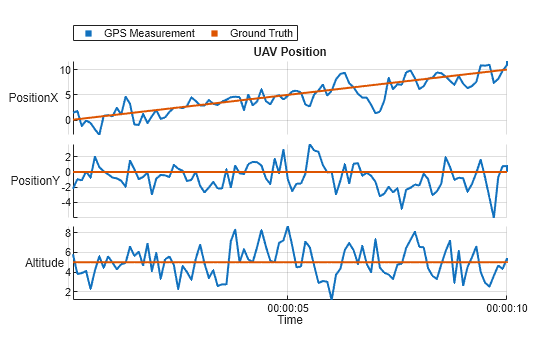
As shown by the ground truth, the UAV is flying at a constant altitude and Y- coordinate, with a X- coordinate that changes at a constant rate. However, because of the measurement noise, the GPS data shows that the UAV position measurement has an erratic change in X- coordinate, changes in Y- coordinate and altitude. This shows that using GPS data by itself is not a reliable method of estimating UAV's position.

Introduction to Kalman Filter

The Kalman filter was primarily developed by the Hungarian engineer Rudolf Kalman, for whom the filter is named. To illustrate the principle of the Kalman filter, consider a scenario in which you are using GPS to navigate while driving.

These figures shows a typical GPS screen. Black squares indicates tall buildings, green indicates open fields, and the blue dot is an estimate of your position.

When you are away from tall buildings, the GPS sensor indicates a small blue dot, indicating a precise position estimate as shown on the left. When you are near tall buildings, however, the GPS position estimate becomes more imprecise, representing a range of possible positions around the blue dot using a transparent blue circle. This range might even suggest you are inside the buildings. However, you instinctively trust the GPS measurement less because you are aware that it is noisy and you know your car is still on the road.

This illustrates the fundamental principle of the Kalman filter: to rely more on sensor measurements as the accuracy of the sensor increases, and rely less on the sensor measurements as the accuracy of the sensor decreases.

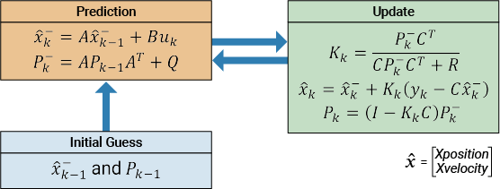
The Kalman filter is an iterative process. After you initialize the filter with an initial guess of the state, the filter performs these operations in each time step of the iteration:

1. Prediction — The filter uses UAV motion models to predict the current state and uncertainty from the previous state.

2. Update — The filter calculates the Kalman gain.

Create Kalman Filter

This diagram illustrates the Kalman Filter algorithm:

State Vector

denotes the state vector of the system. In this simulation, the state vector is as follows:

.

denotes the state vector in iteration step k before the update process, which is also known as the priori state estimate.

denotes the state vector in iteration step k after the update process, which is also known as the posteriori state estimate.

State Transition Matrix

A denotes the state transition matrix, which the filter uses to propagate the state prediction to the next time step.

The state transition matrix depends on the equation of motion that you use to predict the system. In this simulation, the equation of motion is given by:

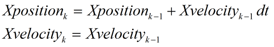
where dt denotes the filter time step size. The matrix representation of this equation is given by:

The state transition matrix is given by:

dt = 1/scenario.UpdateRate;
A = [1 dt;
       0  1];

Since the UAV has no input, you can omit the control matrix and input vector, denoted by B and , respectively. Also, since you know that the equation of motion perfectly describes the UAV motion with no uncertainty, you can omit the process noise matrix denoted by Q.

Estimate Covariance Matrix

denotes the estimate covariance matrix, which stores the uncertainty of the filter state estimate. As an initial guess, assume the filter to have a position estimate variance of 0.5 ${\mathit{m}}^2$ and an initial velocity estimate variance of 0.7 ${\mathit{m}}^2/{\mathit{s}}^2$

Pk_prev = [0.5 0;
           0   0.7];

Observation Matrix

denotes the measurement vector obtained from the GPS sensor. In this simulation, the UAV uses the GPS to measure position.

The observation matrix, denoted by C, determines which measurements the filter uses during its estimation process. Because the filter uses only the GPS position estimate, define the observation matrix as [1 0].

C = [1 0];

Measurement Covariance

R denotes the measurement covariance, which determines measurement uncertainty. Set this parameter to horizontal position variance of the GPS sensor.

R = gpsModel.HorizontalPositionAccuracy^2;

Simulate Kalman Filter

To start the filter, create an initial guess of the state. Assume that the UAV starts at an X-position of 0 meters, with a velocity of 0.5 m/s.

Xk_prev = [0;0.5];

Create a structure array for storing the Kalman filter estimation result.

kalmanFilterData = struct;
kalmanFilterData.Time = gpsData.Time;
kalmanFilterData.PositionX = Xk_prev(1);

Start the Kalman filter.

Nsamples = scenario.StopTime/dt;
for k = 1:Nsamples
    % Predict state
    Xk = A*Xk_prev;
    % Predict P matrix
    Pk = A*Pk_prev*A';
    % Calculate Kalman gain
    S = C*Pk*C' + R;
    K = Pk*C'*inv(S);
    % Obtain measurement data
    y = gpsData.PositionX(k+1);
    % Update state prediction
    Xk = Xk + K*(y-C*A*Xk_prev);
    % Update P matrix prediction
    Pk = Pk - K*C*Pk;  
    % Store data
    Xk_prev = Xk;
    Pk_prev = Pk;
    kalmanFilterData.PositionX = [kalmanFilterData.PositionX; Xk(1)];
end;

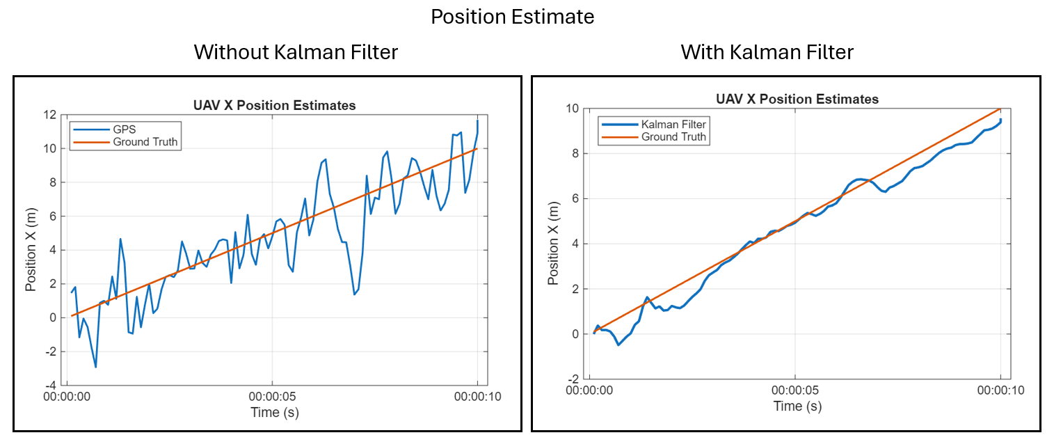
Plot the Kalman filter estimation result along with the GPS-only estimation and the ground truth..

kalmanFilterTimeTable = table2timetable(struct2table(kalmanFilterData));
figure
plot(gpsTimeTable.Time,gpsTimeTable.PositionX,LineWidth=1.5)
hold on
plot(groundTruthTimeTable.Time,groundTruthTimeTable.PositionX,LineWidth=1.5)
hold on
plot(kalmanFilterTimeTable.Time,kalmanFilterTimeTable.PositionX,LineWidth=2)
title("UAV X Position Estimates");
xlabel("Time (s)");
ylabel("Position X (m)");
legend("GPS','Ground Truth','Kalman Filter");
grid on

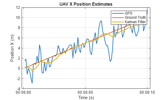
The plot shows that the Kalman filter X position estimate has less noise and less error relative to the ground truth compared to the GPS-only measurement. Therefore, the Kalman filter has improved the position estimate of the UAV.

Modify the Kalman Filter Simulation

You can make modifications to this MATLAB script to experiment with the UAV and Kalman Filter simulation, such as:

• Specify different HorizontalPositionAccuracy and VerticalPositionAccuracy for the GPS sensor.

• Initialize the Kalman filter with a different state and covariance guess by varying the values of Xk_prev and Pk_prev, respectively.

• Use the velocity measurement of the GPS sensor during the estimate update process. For more information on how to obtain GPS velocity measurements, see the gpsSensor.

• Modify the Kalman filter to estimate Y- and Z- positions.

Limitations of Kalman Filter

This example demonstrates a basic Kalman filter, which assumes that the system dynamics and measurement model are linear. This assumption is not valid for a lot of real-world systems. For example, this filter will not be able to estimate the UAV's position if:

• The UAV's velocity is not constant

• The UAV flies in a curved path

• You are using a sensor with a measurement that is not linear to the state you want to estimate, such as radar, which expresses its position measurements in azimuth and range

To estimate the states of systems with high nonlinearity, you must use a Kalman filter that has been adapted to estimate the states of nonlinear systems, such as Extended Kalman Filters (Sensor Fusion and Tracking Toolbox).