Visualize Custom Flight Log
R2026bThis example shows how to configure the flightLogSignalMapping object to visualize flight data from a custom log format. Use this approach when your flight log does not follow a standard ULog or TLog definition and you need to map signals manually before plotting.
Load Custom Flight Log
This example assumes you have already parsed flight data into MATLAB® and stored it as a MAT file. The file customFlightData.mat stores a structure with three fields:
Fs— Sampling frequency of all signalsIMU— Matrix of accelerometer, gyroscope, and magnetometer readingsTrajectory— Matrix of position, velocity, and orientation data
The data is based on a simulated flight that follows a rectangular path on an xy-plane.
customData = load("customFlightData.mat");
logData = customData.logData
logData = struct with fields:
IMU: [2785×9 double]
Fs: 100
Trajectory: [2785×10 double]
The IMU field in logData is an n-by-9 matrix:
Columns 1–3 — Accelerometer readings ()
Columns 4–6 — Gyroscope readings ()
Columns 7–9 — Magnetometer readings ()
logData.IMU(1:5, :)
ans = 5×9

    0.8208    0.7968    10.7424    0.0862    0.0873    0.0862    327.6000    297.6000    283.8000
      ⋮
The Trajectory field in logData is an n-by-10 matrix. Each row represents a single trajectory sample:
Columns 1–3 — XYZ position in the NED frame ()
Columns 4–6 — XYZ velocity in the NED frame ()
Columns 7–10 — Quaternion describing rotation from the NED inertial frame to the body frame
logData.Trajectory(1:5,:)
ans = 5×10

    0.0200    0    -4.0000    2.0000    0    -0.0036    1.0000    0    0    -0.0000
      ⋮
Map and Visualize Predefined Signals
Create a flightLogSignalMapping object with no input arguments, since the custom log format does not follow a standard ULog or TLog definition.
customPlotter = flightLogSignalMapping;
The object defines a set of signals you can map. Mapping these signals gives you access to a set of built-in plots. Some signal names end with a '#' suffix. You can append integers to these names to handle multiple sensors of the same kind, such as secondary IMU signals or barometer readings. To view the available signals and plots, call info.
% Predefined signals
info(customPlotter, "Signal")
ans = 18×4 table
                 "Accel#"    0                                                                                                                                                                                      "AccelX, AccelY, AccelZ"                                  "m/s^2, m/s^2, m/s^2"
              "Airspeed#"    0                                                                                                                                                                   "PressDiff, IndicatedAirSpeed, Temperature"                                     "Pa, m/s, degreeC"
          "AttitudeEuler"    0                                                                                                                                                                                            "Roll, Pitch, Yaw"                                        "rad, rad, rad"
           "AttitudeRate"    0                                                                                                                                                     "BodyRotationRateX, BodyRotationRateY, BodyRotationRateZ"                                  "rad/s, rad/s, rad/s"
    "AttitudeTargetEuler"    0                                                                                                                                                                          "RollTarget, PitchTarget, YawTarget"                                        "rad, rad, rad"
             "Barometer#"    0                                                                                                                                                                        "PressAbs, PressAltitude, Temperature"                                       "Pa, m, degreeC"
                "Battery"    0    "Voltage_1, Voltage_2, Voltage_3, Voltage_4, Voltage_5, Voltage_6, Voltage_7, Voltage_8, Voltage_9, Voltage_10, Voltage_11, Voltage_12, Voltage_13, Voltage_14, Voltage_15, Voltage_16, RemainingCapacity"    "v, v, v, v, v, v, v, v, v, v, v, v, v, v, v, v, %"
                   "GPS#"    0                                                                                                                                  "Latitude, Longitude, Altitude, GroundSpeed, CourseAngle, SatellitesVisible"                  "degree, degree, m, m/s, degree, N/A"
                  "Gyro#"    0                                                                                                                                                                                         "GyroX, GyroY, GyroZ"                                  "rad/s, rad/s, rad/s"
               "LocalENU"    0                                                                                                                                                                                                     "X, Y, Z"                                              "m, m, m"
         "LocalENUTarget"    0                                                                                                                                                                                   "XTarget, YTarget, ZTarget"                                              "m, m, m"
            "LocalENUVel"    0                                                                                                                                                                                                  "VX, VY, VZ"                                        "m/s, m/s, m/s"
      "LocalENUVelTarget"    0                                                                                                                                                                                "VXTarget, VYTarget, VZTarget"                                        "m/s, m/s, m/s"
               "LocalNED"    0                                                                                                                                                                                                     "X, Y, Z"                                              "m, m, m"
      ⋮
% Predefined plots
info(customPlotter,"Plot")
ans = 10×4 table
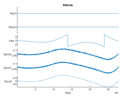
                 "Attitude"    0    "AttitudeEuler, AttitudeRate, Gyro#"    "AttitudeEuler, AttitudeRate, Gyro#"
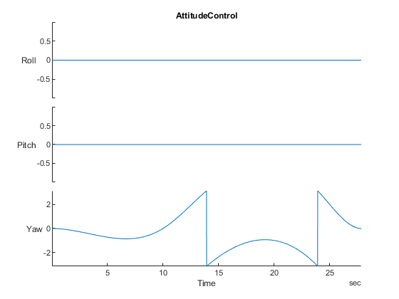
          "AttitudeControl"    0    "AttitudeEuler, AttitudeTargetEuler"    "AttitudeEuler, AttitudeTargetEuler"
                  "Battery"    0                               "Battery"                               "Battery"
                  "Compass"    0             "AttitudeEuler, Mag#, GPS#"             "AttitudeEuler, Mag#, GPS#"
                    "GPS2D"    0                                  "GPS#"                                  "GPS#"
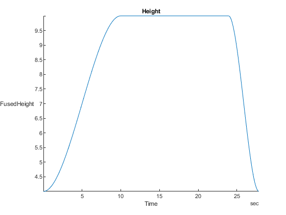
                   "Height"    0            "Barometer#, GPS#, LocalNED"            "Barometer#, GPS#, LocalNED"
                    "Speed"    0                       "GPS#, Airspeed#"                       "GPS#, Airspeed#"
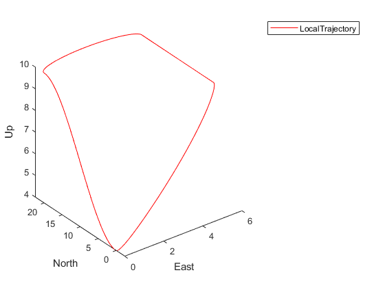
               "Trajectory"    0              "LocalNED, LocalNEDTarget"              "LocalNED, LocalNEDTarget"
       "TrajectoryTracking"    0              "LocalNED, LocalNEDTarget"              "LocalNED, LocalNEDTarget"
    "TrajectoryVelTracking"    0        "LocalNEDVel, LocalNEDVelTarget"        "LocalNEDVel, LocalNEDVelTarget"
The flightLogSignalMapping object needs to know how data is stored in the flight log before it can visualize the data. To associate signal names with function handles that access the relevant information in logData, you must map signals using mapSignal. Each signal is defined as a timestamp vector and a signal value matrix.
For example, to map the Gyro# signal, define a timeAccess function handle based on the sensor data sampling frequency. This function handle generates the timestamp vector for the signal values using a global timestamp interval for the data.
timeAccess = @(x)seconds(1/x.Fs*(1:size(x.IMU)));
Next, check what fields must be defined for the Gyro# signal using info.
info(customPlotter,"Signal","Gyro#")
ans = 1×4 table
    "Gyro#"    0    "GyroX, GyroY, GyroZ"    "rad/s, rad/s, rad/s"
The Gyro# signal needs three columns containing the gyroscope readings for the XYZ axes. Define the gyroAccess function handle accordingly and map it with timeAccess using mapSignal.
gyroAccess = @(x)x.IMU(:,4:6);
mapSignal(customPlotter,"Gyro",timeAccess,gyroAccess);
Similarly, map other predefined signals available in the flight log. Define the value function handles for the data. Map the signals using the same timeAccess timestamp vector function.
% IMU data stores accelerometer and magnetometer data.
accelAccess = @(x)x.IMU(:,1:3);
magAccess = @(x)x.IMU(:,7:9)*1e-2;

% Flight trajectory in local NED coordinates
% XYZ coordinates
nedAccess = @(x)x.Trajectory(:, 1:3);
% XYZ velocities
nedVelAccess = @(x)x.Trajectory(:, 4:6);
% Roll Pitch Yaw rotations converted from a quaternion
attitudeAccess = @(x)flip(quat2eul(x.Trajectory(:, 7:10)),2);

% Configure flightLogSignalMapping for custom data
mapSignal(customPlotter, "Accel", timeAccess, accelAccess);
mapSignal(customPlotter, "Mag", timeAccess, magAccess);
mapSignal(customPlotter, "LocalNED", timeAccess, nedAccess);
mapSignal(customPlotter, "LocalNEDVel", timeAccess, nedVelAccess);
mapSignal(customPlotter, "AttitudeEuler", timeAccess, attitudeAccess);
Once you map all signals, customPlotter can generate plots from the log data. To verify that you mapped signals correctly, call checkSignal and specify logData.
checkSignal(customPlotter,logData);
--------------------------------------------
SignalName: Gyro
Pass
--------------------------------------------
SignalName: Accel
Pass
--------------------------------------------
SignalName: Mag
Pass
--------------------------------------------
SignalName: LocalNED
Pass
--------------------------------------------
SignalName: LocalNEDVel
Pass
--------------------------------------------
SignalName: AttitudeEuler
Pass
To preview a mapped signal, set the Preview option in checkSignal.
checkSignal(customPlotter,logData,Preview="on",Signal="Accel");
--------------------------------------------
SignalName: Accel
Pass
Press a key to continue or 'q' to quit. Figure needs to be in focus.
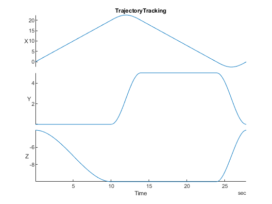
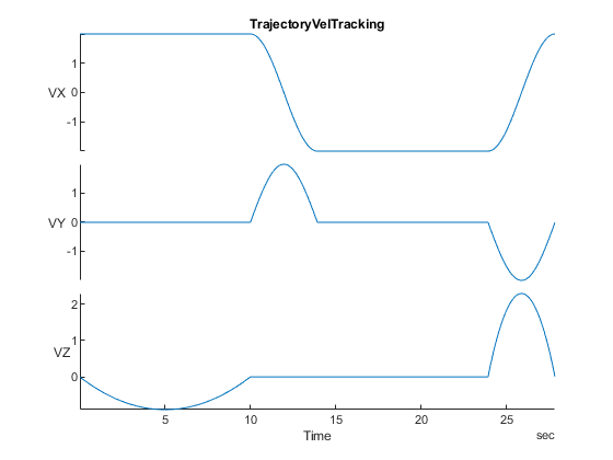
To visualize the flight log data, call show and specify logData. The function generates one figure for each plot that corresponds to the mapped signals.
predefinedPlots = show(customPlotter,logData);

Visualize Custom Flight Log with Custom Plot
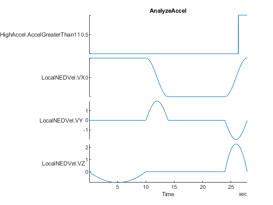
For more detailed log analysis, define additional signals and add custom plots beyond the built-in plots stored in flightLogSignalMapping. Specify a function handle that flags samples where the acceleration norm exceeds 11 m/s².
accelThreshold = @(x) vecnorm(accelAccess(x), 2, 2) > 11;
mapSignal(customPlotter, "HighAccel", timeAccess,accelThreshold, "AccelGreaterThan11", "N/A");
To add custom plots, call updatePlot. Specify the flight log plotter object and a name for the plot as the first two arguments. To specify a time series of data, use "Timeseries" as the third argument, and then list the signals.
updatePlot(customPlotter, "AnalyzeAccel","Timeseries",["HighAccel.AccelGreaterThan11", "LocalNEDVel.VX", "LocalNEDVel.VY", "LocalNEDVel.VZ"]);
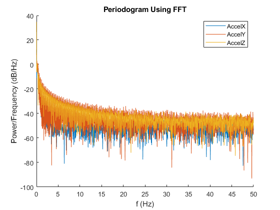
Define a custom plotting function that generates a periodogram of the acceleration data using fft. The function plotFFTAccel (defined at the end of this example) accepts acceleration data and returns a figure handle.
updatePlot(customPlotter, "plotFFTAccel",@(acc)plotFFTAccel(acc),"Accel");
To confirm that customPlotter now contains a new signal and two new plots, call info.
info(customPlotter, "Signal")ans = 19×4 table
"Accel" 1 "AccelX, AccelY, AccelZ" "m/s^2, m/s^2, m/s^2"
"AttitudeEuler" 1 "Roll, Pitch, Yaw" "rad, rad, rad"
"Gyro" 1 "GyroX, GyroY, GyroZ" "rad/s, rad/s, rad/s"
"HighAccel" 1 "AccelGreaterThan11" "N/A"
"LocalNED" 1 "X, Y, Z" "m, m, m"
"LocalNEDVel" 1 "VX, VY, VZ" "m/s, m/s, m/s"
"Mag" 1 "MagX, MagY, MagZ" "Gs, Gs, Gs"
"Airspeed#" 0 "PressDiff, IndicatedAirSpeed, Temperature" "Pa, m/s, degreeC"
"AttitudeRate" 0 "BodyRotationRateX, BodyRotationRateY, BodyRotationRateZ" "rad/s, rad/s, rad/s"
"AttitudeTargetEuler" 0 "RollTarget, PitchTarget, YawTarget" "rad, rad, rad"
"Barometer#" 0 "PressAbs, PressAltitude, Temperature" "Pa, m, degreeC"
"Battery" 0 "Voltage_1, Voltage_2, Voltage_3, Voltage_4, Voltage_5, Voltage_6, Voltage_7, Voltage_8, Voltage_9, Voltage_10, Voltage_11, Voltage_12, Voltage_13, Voltage_14, Voltage_15, Voltage_16, RemainingCapacity" "v, v, v, v, v, v, v, v, v, v, v, v, v, v, v, v, %"
"GPS#" 0 "Latitude, Longitude, Altitude, GroundSpeed, CourseAngle, SatellitesVisible" "degree, degree, m, m/s, degree, N/A"
"LocalENU" 0 "X, Y, Z" "m, m, m"
⋮
info(customPlotter, "Plot")ans = 12×4 table
"AnalyzeAccel" 1 "" "HighAccel, LocalNEDVel"
"Attitude" 1 "AttitudeRate" "AttitudeEuler, AttitudeRate, Gyro#"
"AttitudeControl" 1 "AttitudeTargetEuler" "AttitudeEuler, AttitudeTargetEuler"
"Compass" 1 "GPS#" "AttitudeEuler, Mag#, GPS#"
"Height" 1 "Barometer#, GPS#" "Barometer#, GPS#, LocalNED"
"Trajectory" 1 "LocalNEDTarget" "LocalNED, LocalNEDTarget"
"TrajectoryTracking" 1 "LocalNEDTarget" "LocalNED, LocalNEDTarget"
"TrajectoryVelTracking" 1 "LocalNEDVelTarget" "LocalNEDVel, LocalNEDVelTarget"
"plotFFTAccel" 1 "" "Accel"
"Battery" 0 "Battery" "Battery"
"GPS2D" 0 "GPS#" "GPS#"
"Speed" 0 "GPS#, Airspeed#" "GPS#, Airspeed#"
To visualize the analysis of the acceleration data, call show with "PlotsToShow".
accelAnalysisProfile = ["AnalyzeAccel", "plotFFTAccel"];
accelAnalysisPlots = show(customPlotter, logData, "PlotsToShow", accelAnalysisProfile);
This example shows how to use the flightLogSignalMapping object to visualize predefined signals and create custom plots for flight log analysis.
Supporting Functions
function h = plotFFTAccel(acc)
    h = figure("Name", "AccelFFT");
    ax = newplot(h);
    v = acc.Values{1};
    Fs = v.Properties.SampleRate;
    N = floor(length(v.AccelX)/2)*2;
    hold(ax, "on");
    for col = 1:3
        x = v{1:N, col};
        xdft = fft(x);
        xdft = xdft(1:N/2+1);
        psdx = (1/(Fs*N)) * abs(xdft).^2;
        psdx(2:end-1) = 2*psdx(2:end-1);
        freq = 0:Fs/N:Fs/2;
        plot(ax, freq, 10*log10(psdx));
    end
    hold(ax, "off");
    title("Periodogram Using FFT");
    xlabel("f (Hz)");
    ylabel("Power/Frequency (dB/Hz)");
    legend("AccelX", "AccelY", "AccelZ");
end
See Also
flightLogSignalMapping | mapSignal | updatePlot | show

