Generate DWT Decomposition Using Wavelet Image Analyzer and Share Results

This example shows how to use Wavelet Image Analyzer to visualize the discrete wavelet decomposition of an image and to generate a script to recreate the results in the workspace. The example also shows how to compare two different image reconstructions.

Import Data

You can import an image from your workspace or a file into Wavelet Image Analyzer. Load the xbox image into your workspace.

load xbox

Visualize Wavelet Decomposition

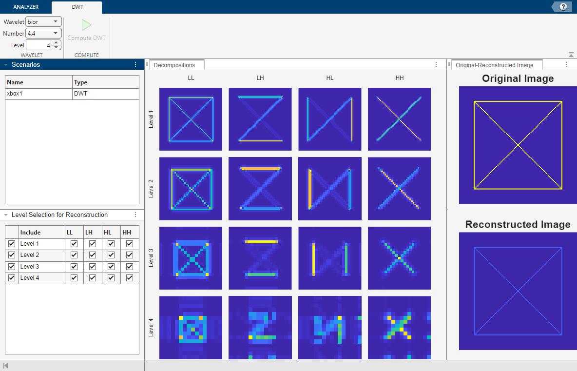
Open Wavelet Image Analyzer. On the Analyzer tab, click Import. A window appears with a list of all the workspace variables that the app can process. Select xbox and click Import. A four-level wavelet decomposition of the image appears and the app switches to the DWT tab. In the Scenarios pane, the decomposition is named xbox1, and the method DWT identifies the kind of decomposition. By default, the decomposition is obtained using the biorthogonal bior4.4 wavelet, which has four vanishing moments each for the decomposition and reconstruction filters.

The column titles in the Decompositions pane refer to the approximation (LL) and details in three orientations: horizontal (LH), vertical (HL), and diagonal (HH). The order of the pair of letters L and H indicates the order in which the app applies the lowpass (L) scaling and highpass (H) wavelet filters to obtain the decomposition at successive levels. For more information about the 2-D DWT algorithm, see wavedec2.

To hide all the plots in a row or column in the Decompositions pane, right-click a plot in that row or column and select the desired action. You can restore all plots, right-click anywhere in the Decompositions pane and select Show complete decomposition.

The check box in the Level Selection for Reconstruction pane controls whether to include those coefficients in the reconstruction. The Original-Reconstructed Image pane shows the original and reconstructed images.

To generate a new decomposition, change one of the wavelet parameters in the toolstrip:

• Wavelet — Wavelet family

• Number — Wavelet filter number

• Level — Wavelet decomposition level

Changing any parameter in the toolstrip enables the Compute DWT button.

Compare DWT Decompositions

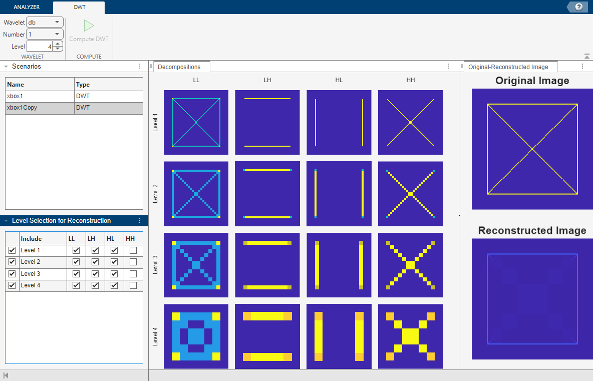
You can create new decompositions of the same signal by clicking either the Add or Duplicate buttons in the Analyzer tab. Changes you make to the wavelet parameters apply only to the selected scenario. Similarly, the coefficients you choose to include in the reconstruction apply only to the selected scenario. To compare decompositions or reconstructions, click the desired scenario in the Scenarios pane.

In the Analyzer tab, click Duplicate. The scenario xbox1Copy appears in the Scenarios panel. Both scenarios decompose the image using the bior4.4 wavelet. In the new scenario, change the wavelet to the Haar (db1) wavelet and decompose. Form the reconstruction using all the coefficients except those corresponding to the diagonal (HH) details.

Export Results

You can either export the image decomposition to your workspace or generate a script to reproduce the results.

To generate a script to recreate the xbox1Copy decomposition in your workspace, in the Analyzer tab, select Export > Generate MATLAB Script.

In the status bar, text appears stating that the script has been generated, and an untitled script opens in your editor with the executable code. You can save the script as is or modify it to apply the same decomposition settings to other images. To create the decomposition in your workspace, save and run the script. The script creates the workspace variable xbox1Copy_DWT. The variable is a structure with the fields:

• transformedImage — This image is the reconstructed image that the app displays in the Original-Reconstructed Image pane.

• decompositionCoefficients — This field corresponds to the wavelet decomposition vector the wavedec2 function returns.

• bookkeepingMatrix — This field corresponds to the bookkeeping matrix the wavedec2 function returns.

If you instead chose to export the image decomposition, the same workspace variable xbox1Copy_DWT is created in your workspace.

Note: If you import an image from a file and export its decomposition, the workspace variable has a fourth structure field, originalImage, which contains the imported image.

% Variables for decomposition and reconstruction
waveletName = "db1";
decompositionLevel = 4;
% Detail gain columns are ordered by LH, HL, HH, rows are ordered by decomposition level
detailGain = [1 1 0;1 1 0;1 1 0;1 1 0];
lowpassGain = 1;

% Perform the decomposition using wavedec2
[C,S] = wavedec2(xbox,decompositionLevel,waveletName);

% Create decompositions by subbands and level
% using the detcoef2 and appcoef2 functions
decompositionTable = table(Size=[decompositionLevel,4], ...
    VariableTypes=["cell","cell","cell","cell"], ...
    VariableNames=["LL","LH","HL","HH"]);

for levelIdx = 1:decompositionLevel
    % Create LH, HL, and HH subbands
    [decompositionTable.LH{levelIdx}, ...
        decompositionTable.HL{levelIdx}, ...
        decompositionTable.HH{levelIdx}] = detcoef2("all",C,S,levelIdx);

    % Create LL subband
    decompositionTable.LL{levelIdx} = appcoef2(C,S,waveletName,levelIdx);
end

% Create reconstructed image using waverec2
reconstructedImage = waverec2(C,S,waveletName, ...
    DetailGain=detailGain,LowPassGain=lowpassGain);

% Create structure for reconstruction data
xbox1Copy_DWT = struct();
xbox1Copy_DWT.transformedImage = reconstructedImage;
xbox1Copy_DWT.decompositionCoefficients = C;
xbox1Copy_DWT.bookkeepingMatrix = S;

% To view coefficients with the "imshow" function, try scaling them with
% the "wcodemat" function. For example:
% >> imshow(uint8(wcodemat(decompositionTable.LH{decompositionLevel},255)));

Compare the original and reconstructed images.

tiledlayout(1,2)
nexttile
imagesc(xbox)
title("Original")
nexttile
im2 = wcodemat(reconstructedImage,255);
imagesc(reconstructedImage)
title("Reconstruction")