Introduction to 5G NR Signal Detection on NI USRP Radio

Since R2024b

This example shows how to deploy a hardware implementation of a 5G NR signal detection algorithm on the FPGA of an NI™ USRP™ radio.

Workflow

In this example, you follow a step-by-step guide to generate a custom FPGA image from a Simulink^® model and deploy it on an NI USRP radio by using a generated MATLAB^® host interface script.

For more information about how to prototype and deploy software-defined radio (SDR) algorithms on the FPGA of an NI USRP radio, see Target NI USRP Radios Workflow.

Design Overview

The algorithm implements a primary synchronization signal (PSS) detector to identify 5G NR signals, then performs orthogonal frequency division multiplexing (OFDM) demodulation using the timing information from the PSS. The result is a synchronization signal block (SSB) signal. The example uses the algorithm from the Introduction to 5G NR Signal Detection (Wireless HDL Toolbox) example and provides an additional wrapper that enables you to generate a bitstream suitable for deployment on the FPGA of an NI USRP radio.

The algorithm transfers the SSB signal to the host through the onboard PL DDR buffer. On the host, you decode the master information block (MIB) from the SSB grid to verify the accuracy of the SSB grid data captured and demodulated on the hardware.

Requirements

To target NI USRP radio devices with Wireless Testbench™, you must install and configure third-party tools and additional support packages.

For details about which NI USRP radios you can target, see Supported Radio Devices.

Note

Generating a bitstream with this workflow is supported only on a Linux^® operating system (OS). For details about host system requirements, see System Requirements.

For details about how to install and configure additional support packages and third-party tools, see Installation for Targeting NI USRP Radios.

Note

If you use this example with a USRP X310 radio with TwinRX daughterboards, you cannot use your radio to transmit a test signal. To verify the design running on your radio by using a transmitted signal, use an external transmitter.

Set Up Environment and Radio

Set up a working directory for running the example by using the openExample function in MATLAB. This function downloads the example files into a subfolder of the Examples folder in the currently running release and then opens the example. If a copy of the example exists, openExample opens the existing version of the example.

openExample("wt/IntroductionTo5GNRSignalDetectionOnNIUSRPRadioExample")

The working directory contains all the files you need to use this example, including helper functions and files. The files you interact with are:

• wtNrDetectionSL.slx — The Simulink hardware generation model. This model includes the design under test (DUT), which is a subsystem that implements a 5G NR signal detection algorithm, and additional subsystems than enable you to simulate the DUT behavior.

• IntroductionTo5GNRSignalDetectionOnNIUSRPRadioExample.m — The MATLAB script that you can use to simulate the behavior of the Simulink model before you generate HDL code.

• Verify5GNRSignalDetectionAlgorithmUsingMATLABExample.m — The live script that you use in MATLAB to verify the algorithm running on your radio.

To program the FPGA on your radio with the bitstream that you generate in this example, and to verify the algorithm running on your radio, use the Radio Setup wizard to connect and set up your radio.

Simulink Hardware Generation Model

The Simulink model in this example is a hardware generation model of an SDR algorithm. Using the HDL Code tab in the Simulink Toolstrip or the HDL Workflow Advisor, you can generate a custom HDL IP core from the model, then generate a bitstream and load it onto the FPGA on your radio. You can then generate a host interface script that provides the MATLAB code you need to interact with the hardware.

Open Model

The Simulink model implements the signal detection and demodulation algorithm using a hardware modeling style and uses blocks that support HDL code generation. It uses fixed-point arithmetic and includes control signals that control the flow of data through the model.

Open the model from MATLAB.

open_system('wtNrDetectionSL');

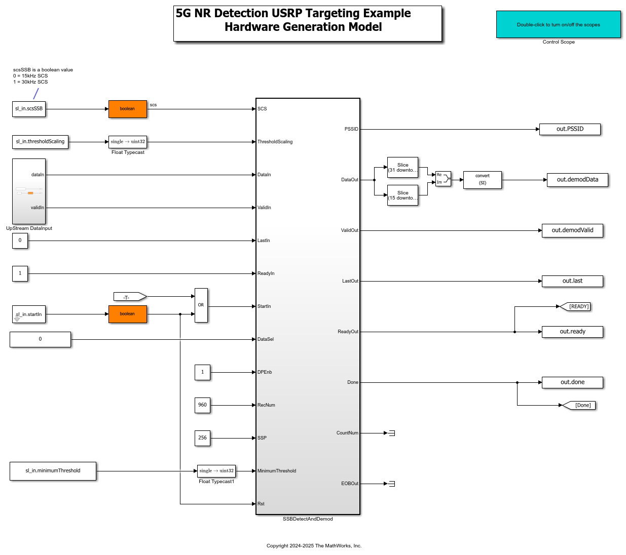
The top level model generates input data for and reads output data from the SSBDetectAndDemod subsystem.

Open the SSBDetectAndDemod subsystem. This subsystem is the DUT that you generate HDL code for in this example.

open_system('wtNrDetectionSL/SSBDetectAndDemod');

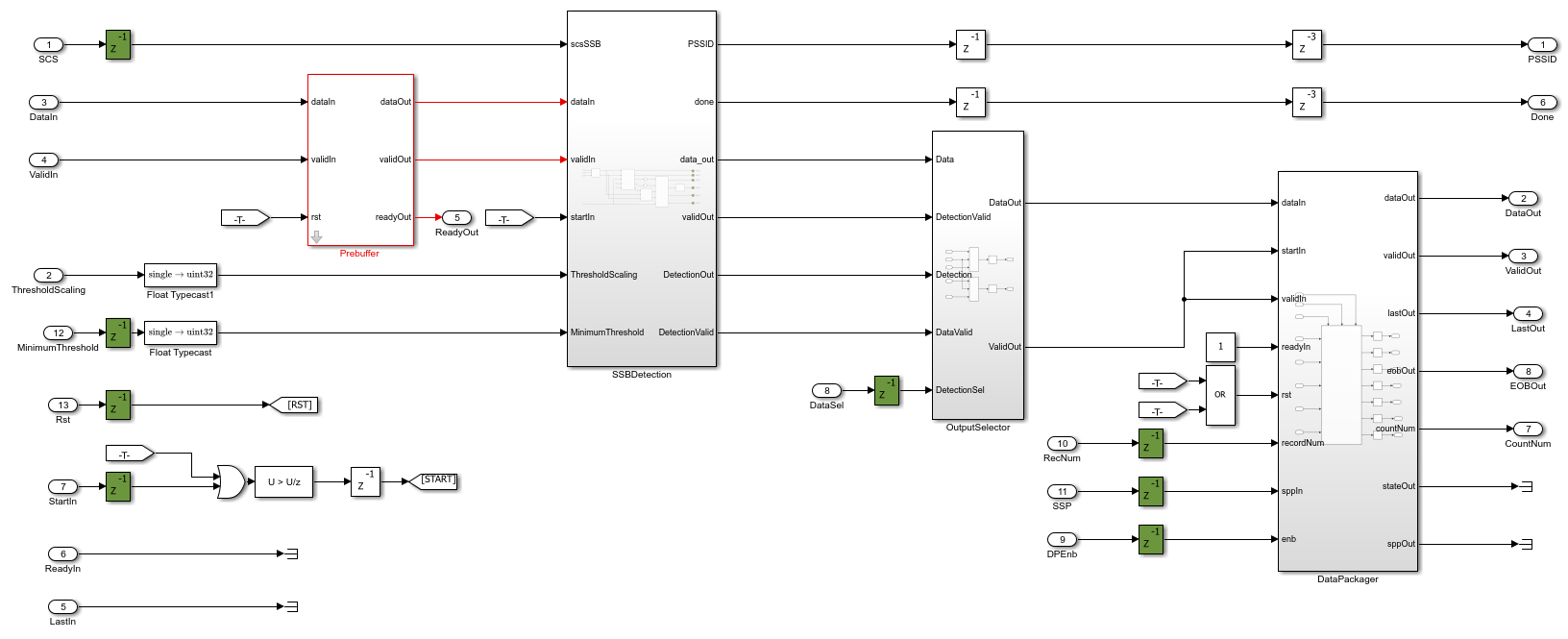
Data flows through these blocks and subsystems:

• The Prebuffer block buffers and reshapes input samples.

• The SSBDetection subsystem detects and demodulates a PSS and outputs the SSB.

• The OutputSelector subsystem processes the SSB and selects the data to stream out.

• The DataPackager subsystem reformats the output samples.

The Prebuffer block and Data Packager subsystem enable rapid development by reformatting the input and output data to conform with the AXI-Stream protocol required by NI USRP radio device reference design. These blocks are in the targetingLib.slx library. You can find the location of this library by using this MATLAB command:

>> which targetingLib

The timing diagram shows how the Prebuffer block reformats the input data samples so that they are output at consistent clock cycle intervals. The reformatting facilitates the reuse of DSP within the SSBDetection subsystem.

The Data Packager subsystem formats the raw streams of output data into the AXI-Stream format. The output packet length is 256 samples, which is the recommended value. The timing diagram shows the inputs and the output, where the output signals conform to the simplified AXI-stream protocol. For more information, see Simplified AXI-Stream Protocol.

The OutputSelector subsystem routes either the cross-correlation data and threshold values or the demodulated signal to the Data Packager subsystem. You can select between these outputs by writing either 0 or 1 to the DataSel port.

Open the SSBDetection subsystem.

open_system('wtNrDetectionSL/SSBDetectAndDemod/SSBDetection');

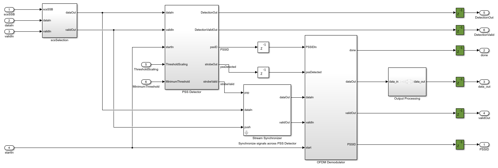
The SSBDetection subsystem detects a PSS signal and then demodulates the SSB. You can select to output the cross-correlation data alongside threshold values for visualization purposes, or to output the demodulated SSB signal for decoding. The adaptive threshold and minimum threshold are adjustable. You can configure these values by writing a numerical value to the ThresholdScaling and MinimumThreshold ports.

Simulate Design

Verify the design by simulating the model.

Set the cell ID to 1.

NCellID = 1;

Set the SSB subcarrier spacing, scsSSB, based on the SSB pattern. SSB pattern Case A uses 15 kHz subcarrier spacing. SSB patterns Case B and Case C use 30 kHz subcarrier spacing.

scsSSB = 30;

Initialize the constants required by the Simulink model.

sl_in = Nr5GDetectionSimSetup(NCellID, scsSSB);

Simulate the model.

sl_out = sim("wtNrDetectionSL.slx");

Process the simulation output data.

sl_demod = sl_out.demodData(sl_out.demodValid);
demoCellID = sl_out.PSSID(find(sl_out.demodValid, 1));
sl_SSBGrid = reshape(sl_demod,240,[]);
numTB = size(sl_SSBGrid,2)/4;

You can use this scope to view the cross-correlation and threshold values during the simulation. The display shows PSS0 correlation peaks are detected during every burst.

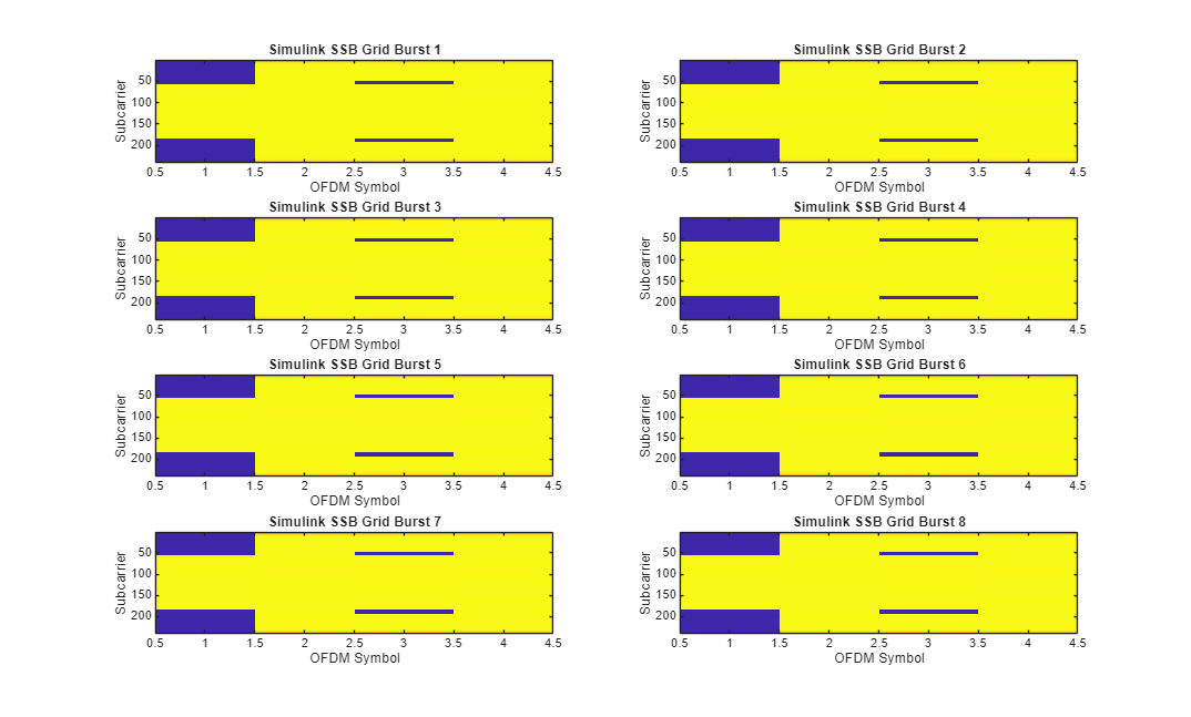
Decode and plot the demodulated data.

fprintf('Decoding MIB from Simulink SSB grid \n');

Decoding MIB from Simulink SSB grid 

Lmax = 8;
figure;
for ii = 0:numTB-1
    startIndex = ii * 4 + 1;
    finishIndex = (ii+1)* 4;
    sl_SSBGridBurst = sl_SSBGrid(1:240, startIndex:finishIndex);
    [~, nCellID, ssbIndex, bchCRC(ii+1)] = ...
        mibDecode(sl_SSBGridBurst, double(demoCellID), Lmax); %#ok<SAGROW>
    subplot(4,2,ii+1)
    imagesc(abs(sl_SSBGridBurst));
    title(['Simulink SSB Grid Burst ', num2str(ii+1)])
    ylabel('Subcarrier');
    xlabel('OFDM Symbol');
end
if(any(bchCRC))
    fprintf('MIB decode failed, bchCRC was nonzero\n');
else
    fprintf('MIB decode successful\n');
end

MIB decode successful

Configure IP Core

When you are satisfied with the simulated behavior of the model, you can proceed to integrate your design into a custom IP core by generating HDL code and mapping the model inputs and outputs to the hardware interfaces.

First, use the hdlsetuptoolpath (HDL Coder) function to set up the tool chain. Specify the path to your Vivado^® bin directory. For more information, see Set Up Third-Party Tools.

hdlsetuptoolpath('ToolName','Xilinx Vivado', ...
    'ToolPath','/opt/Xilinx/Vivado/2021.1/bin');

From the Apps tab in the Simulink Toolstrip, select HDL Coder. Then open the HDL Code tab.

Configure Output Options

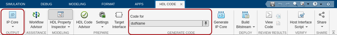
In the HDL Code tab, configure the output options:

• Ensure the SSBDetectAndDemod subsystem is pinned in the Code for option. To pin this selection, select the SSBDetectAndDemod subsystem in the Simulink model and click the pin icon.

• Select IP Core as the Output > IP Core option.

Configure HDL Code Generation Settings

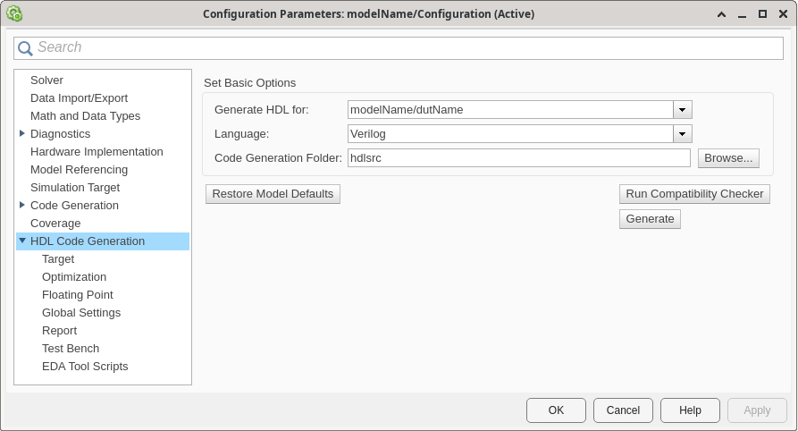
Open the Configuration Parameters dialog box by clicking Settings in the HDL Code tab.

In the HDL Code Generation pane, ensure that Language is set to Verilog. By default, HDL Coder generates the Verilog^® files in the hdlsrc folder. You can select an alternative location. If you make any changes, click Apply.

In the Target pane, configure these settings:

• Under Workflow Settings, select the IP Core Generation workflow. To set Project Folder, click Browse and select a target location for saving the generated project files. If you do not specify a project folder, the software saves the generated project files in the working directory.

• Under Tool and Device Settings, select your radio from the Target Platform list. This example uses a USRP N320 radio. If you are using a different radio, adjust the reference design parameters accordingly.

• Under Reference Design Settings, set Reference Design to the desired reference FPGA image for your design, based on how you set up your hardware. For a USRP N320 radio, you have one option: HG: 1 GigE, 10 GigE.

  Set the reference design parameters to these values:

  • Number of Input Streams — Set to 1 because the DUT is connected to one data input stream from the radio.

  • Number of Output Streams — Set to 1 because the DUT is connected to one data output stream to the host.

  • Sample Rate (S/s) — Set to 7.68e6, which is the bandwidth of the SSB in the 5G downlink signal. To determine which sample rates are available for your radio, see Determine Radio Device Capabilities.

  • Reference Design Optimization — Set to None. The design in this example does not require optimizations to meet timing constraints.

  • DUT Clock Source — Set to Radio. When you select this setting, the DUT is clocked at the MCR used by the radio to achieve the specified sample rate. Alternatively, you can set this setting to Custom to set the DUT clock frequency to a user-defined value in the Target Frequency parameter under Objectives Settings.

  • Stream Port FIFO Length (Samples) — Set to Auto. This setting automatically calculates the buffer length for each DUT input and output data streaming port.

  • Register Port FIFO Length (Samples) — Set to Auto. This setting automatically calculates the buffer length for each DUT register port.

  Under Objectives Settings, since the DUT Clock Source is set to Radio, the Target Frequency is fixed at the highest supported MCR of the radio.

Click Apply.

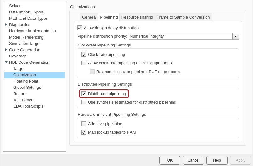
In the Optimization pane, select Distributed pipelining.

In the Floating Point pane, select Use Floating Point.

To apply these settings and close the Configuration Parameters window, click OK.

For more information, see Configure HDL Code Generation Settings.

Map Target Interfaces

In the HDL Code tab, click Target Interface to open the Interface Mapping table in the IP Core editor. To populate the table with your user logic, click the Reload IP core settings button: .

The Source, Port Type, and Data Type columns are populated based on the Simulink model. The Interface column automatically populates based on the port names in your model:

• The input register ports map to Write Register interfaces.

• The output register ports map to Read Register interfaces.

• The DataIn, ValidIn, LastIn, and ReadyOut ports map to a Simplified AXI4-stream Input0 interface.

• The DataOut, ValidOut, LastOut, EOBOut, and ReadyIn ports map to a Simplified AXI4-stream Output0 interface.

The Interface Mapping column is populated automatically based on the port names in the model.

To set the interface options for the streaming interfaces, open the Set Interface Options window by clicking Options in the far right of the table.

For the DataIn options, select a receive antenna as the source connection. The DUT receives input samples from this antenna on the radio. Set the stream buffer size to 32768, which is the default setting. The buffer size must be a power of two to ensure optimal use of the FPGA RAM resources. The buffer size is specified in terms of the number of samples, with each sample having a size of 8 bytes.

For the DataOut options, select the PL DDR buffer as the sink connection. The DUT streams samples first to the onboard radio memory buffer, then to MATLAB for post-processing.

When you have populated the table, validate the interface mapping by clicking the Validate IP core settings button: .

For more information, see Map Target Interfaces.

Generate and Load Bitstream

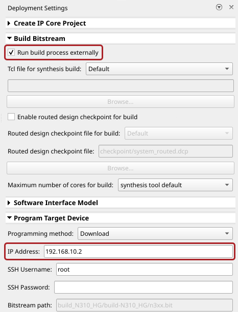
To generate a bitstream from the configured IP core, first open the deployment settings from the Build Bitstream button.

• Ensure that the Run build process externally option is selected. This setting is the default and it ensures that the bitstream build executes in an external shell, which allows you to continue using MATLAB while building the FPGA image.

• In the Program Target Device settings, set the IP address. The default is 192.168.10.2. If your radio has a different IP address, update this field with the correct value.

Click Build Bitstream to create a Vivado IP core project and build the bitstream. After the basic project checks complete, the Diagnostic Viewer displays a Build Bitstream Successful message along with warning messages. However, you must wait until the external shell displays a successful bitstream build before moving to the next step. Closing the external shell before this time terminates the build.

The bitstream for this project generates with the name n3xx.bit and is located in the build_N320_HG/build_N320_HG folder of the working directory after a successful bitstream build. If you are using a different radio, the name and location reflects your radio.

To load the bitstream onto the device now, click Program Target Device from the Build Bitstream button. Alternatively, you can load the bitstream later by using the programFPGA function in the generated host interface script.

For more information, see Generate Bitstream and Program FPGA.

Generate Host Interface Scripts

To generate MATLAB scripts that enable you to connect to and run your deployed design on your radio, in the HDL Code tab, click Host Interface Script. This step generates two scripts in your working directory based on the target interface mapping that you configured for your IP core.

• gs_wtNrDetectionSL_interface.m — Host interface script that creates an fpga object for interfacing with your DUT running on the FPGA from MATLAB. The script contains code that connects to your hardware and programs the FPGA and code samples to get you started with running the algorithm on your radio. For more information, see Interface Script File.

• gs_wtNrDetectionSL_setup.m — Setup function that configures the fpga object with the hardware interfaces and ports from your DUT algorithm. The function contains DUT port objects that have the port name, direction, data type, and interface mapping information, which it maps to the corresponding interfaces. For more information, see Setup Function File.

Edit Setup Function File

In the generated setup function file, the streaming interfaces are configured with the default frame size, which is 1e5 samples. The model in this example uses a frame size of 1e7. Before you run the host interface script, manually update the frame size to 1e7 by following these steps.

1. Open the setup function file for editing.

   edit gs_wtNrDetectionSL_setup.m

2. Identify the call to the addRFNoCStreamInterface function for the data output port.

3. Update the FrameSize value to 1e7.

   RX_STREAM0_FrameSize = 1e7;

4. Save the updated setup function file.

Verify 5G NR Signal Detection Algorithm Using MATLAB

To verify the algorithm running on your radio, use this modified version of the host interface script to transmit a 5G NR test waveform from MATLAB, read the demodulated data from the DUT, and decode and visualize the data.

Open Live Script

You can open this live script in MATLAB from the example working directory and use it interactively. In the Files panel, navigate to your example working directory and open Verify5GNRSignalDetectionAlgorithmUsingMATLABExample.m.

Select Radio

Call the radioConfigurations function. The function returns all available radio setup configurations that you saved using the Radio Setup wizard.

savedRadioConfigurations = radioConfigurations;

To update the menu with your saved radio setup configuration names, click Update. Then select the radio to use with this example.

savedRadioConfigurationNames = [string({savedRadioConfigurations.Name})];
radio = savedRadioConfigurationNames(1) ;

Evaluate the transmit and receive antennas available on your radio device. You select transmit and capture antenna connections for exercising your DUT from the available options later in the script.

receiveAntennas = hCaptureAntennas(radio);
transmitAntennas = hTransmitAntennas(radio);

Create usrp System Object

Create a usrp System object™ with the specified radio. This System object controls the radio hardware.

device = usrp(radio);

Program FPGA

If you have not yet programmed your device with the bitstream, select the load bitstream option to use the programFPGA function. Update the code with your bitstream and device tree file. You can find these files in the programFPGA call in the generated host interface script, gs_wtNrDetectionSL_interface. If your radio is a USRP X310, you need only a bitstream file to program the FPGA.

loadBitstream = false;
if(loadBitstream)
    programFPGA(device, ...
        "build_N320_HG/build-N320_HG/n3xx.bit", ...     % replace with your .bit file
        "build_N320_HG/build/usrp_n320_fpga_HG.dts");   % replace with your .dts file
end

To configure the DUT interfaces according to the hand-off information file, use the describeFPGA function. Calling this function additionally sets the default values for the SampleRate, DUTInputAntennas, and DUTOutputAntennas properties based on the selections you made in Simulink.

% Replace with your hand-off information file
describeFPGA(device, ...
"wtNrDetection/wtNrDetectionSL_wthandoffinfo.mat");

Configure Device

Configure the usrp System object to specify the sample rate, receive center frequency, and antenna gain values. The design requires an input sample rate of 7.68 MSPS.

device.SampleRate = 7.68e6;
device.ReceiveCenterFrequency = 2.4e9;
device.TransmitRadioGain = 30;
device.ReceiveRadioGain = 30;

Specify an available receive antenna to connect to your DUT.

device.DUTInputAntennas = receiveAntennas(1);

Specify a transmit antenna for transmitting a test waveform to exercise the DUT.

device.TransmitAntennas = transmitAntennas(2); 

Create and Set Up FPGA Object

To connect to the DUT on the FPGA of your radio, create an fpga object with the your usrp System object device.

dut = fpga(device);

Set up the fpga object using the generated setup function, gs_wtNrDetectionSL_setup. If you have not updated this file to set the frame size to 1e7, return to Edit Setup Function File.

gs_wtNrDetectionSL_setup(dut);

Set Up Device Object

To establish a connection with the radio hardware, call the setup function on the usrp System object. This action connects to the radio, applies the radio front end properties, and validates that the bitstream file matches the hand-off information file.

setup(device);

Repeatedly Transmit Test Waveform

Generate a test waveform using the hWaveGenHw helper function. The helper function generates a basic 5G waveform using the nrWaveformGenerator function from 5G Toolbox™. For more information about generating 5G waveforms, see 5G NR Downlink Vector Waveform Generation (5G Toolbox).

Choose a cell ID in the range 0 to 1007.

NCellID = 2;

Set scsSSB to 30 to generate a waveform with SSB pattern Case C and a subcarrier pacing of 30 kHz. To generate a waveform with SSB pattern Case A and a subcarrier spacing of 15 kHz, set scsSSB to 15.

scsSSB = 30;

Use the hWaveGenHW helper function to generate an SSB with a period of 5 ms. A 5 ms period is used to make it easier to view a detailed signal in the spectrogram. The standard SSB period is 20 ms.

scaledSigIn = hWaveGenHw(scsSSB,NCellID);

Repeatedly transmit the waveform from the selected transmit antennas by calling the transmit function in continuous mode.

transmit(device,scaledSigIn,"continuous");
writePort(dut,"SCS",scsSSB==30);

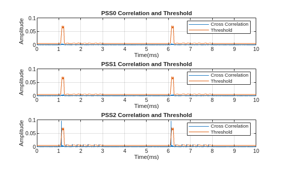
Plot Cross Correlation and Threshold

The detection results depend on the threshold scaling and minimum threshold values. Plot the PSS correlation peaks and PSS threshold from the hardware and use the plots to tune these values. Set the MinimumThreshold to a value that is above the noise floor. Adjust the ThresholdScaling and plot the threshold information repeatedly until the one of the correlator outputs is greater than the adaptive threshold.

Set the plot length to 10 ms. This is more than twice the length of the transmitted signal.

To show the cross-correlation results and adaptive threshold, click Plot.

plotConfig.ThresholdScaling = -4.55; % Strength threshold in dBs (0 is least sensitive).
plotConfig.MinimumThreshold = -23; % Minimum threshold in dBs (0 is least sensitive).
plotConfig.PlotLength = 10;  % milliseconds
 
hPlotXCorrThreshold(dut,device,plotConfig);

Detect NR Signal and Decode

Decode the MIB from the SSB grid to further verify data recovered from the signal. If the bchCRC returned is 0 this indicates no errors are found.

[demodData, PSSID] = hReadDemodData(dut, device);
hardware_SSBGrid = reshape(demodData,240,[]);
Lmax = 8;
[mibStruct, nCellID, ssbIndex, bchCRC] = mibDecode( ...
hardware_SSBGrid(1:240,:),double(PSSID),Lmax);
if(logical(bchCRC))
    fprintf('MIB decode failed, bchCRC is nonzero\n');
else
fprintf('MIB decode successful\n');
fprintf('Cell identity: %d \n', nCellID);
end

MIB decode successful

 Cell identity: 2 

Release Hardware Resources

Stop the transmission and release the hardware resources.

stopTransmission(device);
release(dut);
release(device);