Simulate an 802.11ax Network with Uplink and Downlink Application Traffic
This example shows how to create, configure, and simulate an IEEE® 802.11ax™ (Wi-Fi 6) network with uplink (UL) and downlink (DL) application traffic.
Using this example, you can:
Create and configure an 802.11ax network consisting of an access point (AP) and a station (STA).
Associate the STA with the AP.
Generate, configure, and add UL and DL on-off application traffic between the STA and the AP.
Simulate the 802.11ax network and visualize the statistics.
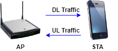
The example simulates this scenario.
Check if the Communications Toolbox™ Wireless Network Simulation Library support package is installed. If the support package is not installed, MATLAB® returns an error with a link to download and install the support package.
wirelessnetworkSupportPackageCheck;
Set the seed for the random number generator to 1. The seed value controls the pattern of random number generation. The random number generated by the seed value impacts several processes within the simulation including backoff counter selection at the MAC layer and predicting packet reception success at the physical layer. To improve the accuracy of your simulation results, after running the simulation, you can change the seed value, run the simulation again, and average the results over multiple simulations.
rng(1,"combRecursive");Specify the simulation time in seconds.
simulationTime = 0.2;
Initialize the wireless network simulator.
networkSimulator = wirelessNetworkSimulator.init;
Set the positions of the AP and the STA as a 2-by-1 vector. Units are in meters. Each row of the vector specifies the x-, y-, and z- Cartesian coordinates of a node, starting from the first node.
nodePositions = [0 0 0;0 -20 0];
Set the configuration parameters of the AP and the STA by using the wlanDeviceConfig object.
accessPointCfg = wlanDeviceConfig(Mode="AP",MCS=2,TransmitPower=15);    % AP device configuration
stationCfg = wlanDeviceConfig(Mode="STA",MCS=2,TransmitPower=15);       % STA device configuration
Create an AP and a STA from the specified configuration by using the wlanNode object.
accessPoint = wlanNode(Name="AP", ...
    Position=nodePositions(1,:), ...
    DeviceConfig=accessPointCfg);

stations = wlanNode(Name="STA", ...
    Position=nodePositions(2,:), ...
    DeviceConfig=stationCfg);
Create an 802.11ax network consisting of an AP and a STA.
nodes = [accessPoint stations];
Associate the STA with the AP.
associateStations(accessPoint,stations);
Generate an on-off application traffic pattern by using the networkTrafficOnOff object. Configure the on-off application traffic by specifying the application data rate and packet size. Add UL and DL application traffic between the AP and the STA by using the addTrafficSource object function.
Alternatively, you can configure full buffer application traffic between the APs and STAs by using the FullBufferTraffic input of the associateStations object function.
trafficSourceUL = networkTrafficOnOff(DataRate=100000,PacketSize=1500);
addTrafficSource(stations,trafficSourceUL,DestinationNode=accessPoint,AccessCategory=0); % UL traffic from STA to AP

trafficSourceDL = networkTrafficOnOff(DataRate=100000,PacketSize=1500);
addTrafficSource(accessPoint,trafficSourceDL,DestinationNode=stations,AccessCategory=0); % DL traffic from AP to STA
Add nodes to the wireless network simulator.
addNodes(networkSimulator,nodes);
Run the network simulation for the specified simulation time.
run(networkSimulator,simulationTime);
At each node, the simulation captures the statistics by using the statistics object function. The stats variable captures the application statistics, MAC layer statistics, physical layer statistics, and mesh forwarding statistics for each node. For more information about these statistics, see the WLAN System-Level Simulation Statistics topic.
stats = statistics(nodes)
stats=1×2 struct array with fields:
    Name
    ID
    App
    MAC
    PHY
    Mesh
See Also
Functions
Objects
Related Topics
You can also select a web site from the following list:
Americas
- América Latina (Español)
- Canada (English)
- United States (English)
Europe
- Belgium (English)
- Denmark (English)
- Deutschland (Deutsch)
- España (Español)
- Finland (English)
- France (Français)
- Ireland (English)
- Italia (Italiano)
- Luxembourg (English)
- Netherlands (English)
- Norway (English)
- Österreich (Deutsch)
- Portugal (English)
- Sweden (English)
- Switzerland
- United Kingdom (English)