Sensitivity Analysis of Epidemic ODE Parameters

This example shows how to perform sensitivity analysis on the parameters of an ordinary differential equation (ODE) system that models the spread of a disease in an epidemic.

SIR Epidemic Model

A simple SIR model for epidemic spread [1] assigns members of the population to three groups (S, I, and R). As the simulation progresses, people can move between the groups. The model can predict outcomes for human-to-human transmission of infectious diseases where recovered individuals are able to resist further infection.

• S — The number of susceptible people. Susceptible people can transition into the infected group if they come into contact with an infected person.

• I — The number of infected people. Members of this group are capable of infecting people in the susceptible group.

• R — The number of recovered people who were previously infected with the disease. Members of this group are immune from further infection.

The SIR model can be expressed with a system of three first-order ODEs:

$$\begin{array}{l}\frac{\mathrm{dS}}{\mathrm{dt}}=-\beta \frac{\mathrm{IS}}{\mathit{N}},\\ \frac{\mathrm{dI}}{\mathrm{dt}}=\beta \frac{\mathrm{IS}}{\mathit{N}}-\gamma \mathit{I},\\ \frac{\mathrm{dR}}{\mathrm{dt}}=\gamma \mathit{I}.\end{array}$$

The variable $\mathit{N}$ represents the total population $\mathit{N}=\mathit{S}+\mathit{I}+\mathit{R}$. The model also uses two parameters, $\beta$ and $\gamma$. The $\beta$ parameter specifies the average number of contacts with infected people multiplied by the probability of disease transmission. The $\gamma$ parameter specifies how quickly people recover from the disease. If a person is infectious for $\mathit{d}$ days, then $\gamma =1/\mathit{d}$. The strength of disease spread depends on the ratio of the parameters $\beta /\gamma$. This quantity is also called the reproduction number, and it describes the number of new infections expected from a single infection in the population. A large reproduction number means that people contract the disease much faster than they recover.

The initial conditions describe the initial populations in each group. For this example, the initial conditions are:

$$\begin{array}{l}\mathit{S}\left(0\right)=995,\\ \mathit{I}\left(0\right)=5,\\ \mathit{R}\left(0\right)=0.\end{array}$$

That is, there are initially 995 people susceptible to infection, 5 infected people, and 0 people with immunity who have recovered.

Code Equations

To simulate the system, create a function epidemic(t,y,p) that encodes the equations and returns the population change for each group at each time step. Specify three inputs to the function to pass in the parameter values p from the workspace.

function dydt = epidemic(t,y,p)
    beta = p(1);
    gamma = p(2);

    S = y(1);
    I = y(2);
    R = y(3);
    N = S + I + R;

    dSdt = -beta*(I*S)/N;
    dIdt = beta*(I*S)/N - gamma*I;
    dRdt = gamma*I;

    dydt = [dSdt;
            dIdt;
            dRdt];
end

Create ode Object

Specify parameter values of $\beta =0.4$ and $\gamma =0.04$. These parameter values give a reproduction number of $\beta /\gamma =10$. Also create a vector of initial conditions $\left[99550\right]$. Finally, create an ode object to represent the problem, specifying the equations, initial conditions, and parameter values.

p1 = [0.4 0.04];
ic = [995 5 0];
F = ode(ODEFcn=@epidemic, ...
        InitialValue=ic, ...
        Parameters=p1);

Simulate and Plot Results

Simulate the system of equations over the time interval [0 80]. Plot the resulting populations over time.

sol1 = solve(F,0,80)

sol1 = 
  ODEResults with properties:

        Time: [0 2.5119e-04 5.0238e-04 7.5357e-04 0.0010 0.0023 0.0035 0.0048 0.0060 0.0123 0.0186 0.0249 0.0311 0.0625 0.0939 0.1253 0.1567 0.3137 0.4707 0.6277 0.7847 1.2565 1.7284 2.2002 2.6720 3.3211 3.9702 4.6193 5.2684 6.0288 ... ] (1x93 double)
    Solution: [3x93 double]

plot(sol1.Time,sol1.Solution,"-o")
legend("S","I","R")
title(["SIR Populations over Time","$\beta=0.4$, $\gamma=0.04$"],Interpreter="latex")
xlabel("Time",Interpreter="latex")
ylabel("Population",Interpreter="latex")

With these parameter values, the population of infected people has a large peak around $\mathit{t}=25$, indicating that the disease spreads quickly and infects much of the susceptible population.

Change the parameter values to $\beta =0.2$ and $\gamma =0.1$, which reduces the reproduction number to $\beta /\gamma =2$. Also specify set the Sensitivity property of the ode object to an odeSensitivity object to enable sensitivity analysis of the parameters. Sensitivity analysis examines how sensitive the equations are to changes in the parameter values. Simulate the system with the new parameters and plot the results.

p2 = [0.2 0.1];
F.Parameters = p2;
F.Sensitivity = odeSensitivity;
sol2 = solve(F,0,80)

sol2 = 
  ODEResults with properties:

           Time: [0 1.8323e-08 1.8324e-04 0.0014 0.0027 0.0083 0.0138 0.0693 0.1703 0.2713 0.5478 0.8243 1.7724 2.7205 4.2160 5.7116 7.2071 10.3457 13.4843 16.6229 19.7615 22.9001 26.0387 29.1773 32.3159 35.4545 38.5931 41.7317 44.8703 ... ] (1x48 double)
       Solution: [3x48 double]
    Sensitivity: [3x2x48 double]

plot(sol2.Time,sol2.Solution,"-o")
legend("S","I","R")
title(["SIR Populations over Time","$\beta=0.2$, $\gamma=0.1$"],Interpreter="latex")
xlabel("Time",Interpreter="latex")
ylabel("Population",Interpreter="latex")

In this case, the disease spreads much more slowly, and not all of the susceptible people get infected within the same period of time.

Examine Parameter Sensitivity

Sensitivity analysis examines how changes in parameter values can affect the solution of the ODE. When the Sensitivity property of an ode object is nonempty, the solver performs sensitivity analysis on the parameters you specify (by default, all parameters). The ODEResults object returned by the call to solve contains an extra property, Sensitivity, that contains partial derivative values of the equations with respect to the parameters.

Consider an ODE system of the form

$$\frac{{\mathrm{dy}}_{\mathit{i}}}{\mathrm{dt}}={\mathit{f}}_{\mathit{i}}\left(\mathit{t},\mathit{y},\mathit{p}\right),\mathit{i}=1,2,...,\mathit{n}.$$

The parameters $\mathit{p}$ can be treated as independent variables to obtain the sensitivity functions

$${\mathit{u}}_{\mathrm{ij}}=\frac{{\partial \mathit{y}}_{\mathit{i}}}{{\partial \mathit{p}}_{\mathit{j}}},\mathit{i}=1,2,...,\mathit{n},\mathit{j}=1,2,...,\mathit{m}.$$

The variable $\mathit{i}$ represents the number of equations in the system, and $\mathit{j}$ represents the number of parameters being analyzed. The Sensitivity property of the ODEResults object contains these partial derivative values for ${\mathit{u}}_{\mathrm{ij}}$. The size of the Sensitivity array is:

(Number of equations)-by-(Number of parameters)-by-(Number of time steps)

One common use of the sensitivity functions is to compute the normalized sensitivity functions [2], which describe the approximate percentage change in each solution component due to a small change in the parameter. You can calculate the normalized sensitivity functions using ${\mathit{u}}_{\mathrm{ij}}$, the calculated solution ${\mathit{y}}_{\mathit{i}}$, and the parameter values ${\mathit{p}}_{\mathit{j}}$.

$${\mathit{U}}_{\mathrm{ij}}={\mathit{u}}_{\mathrm{ij}}\frac{{\mathit{p}}_{\mathit{j}}}{{\mathit{y}}_{\mathit{i}}}$$

Calculate the normalized sensitivity functions using sol2.Sensitivity as well as the computed solution sol2.Solution and the parameter values p2 = [0.2 0.1].

U11 = squeeze(sol2.Sensitivity(1,1,:))'.*(p2(1)./sol2.Solution(1,:));
U12 = squeeze(sol2.Sensitivity(1,2,:))'.*(p2(2)./sol2.Solution(1,:));
U21 = squeeze(sol2.Sensitivity(2,1,:))'.*(p2(1)./sol2.Solution(2,:));
U22 = squeeze(sol2.Sensitivity(2,2,:))'.*(p2(2)./sol2.Solution(2,:));
U31 = squeeze(sol2.Sensitivity(3,1,:))'.*(p2(1)./sol2.Solution(3,:));
U32 = squeeze(sol2.Sensitivity(3,2,:))'.*(p2(2)./sol2.Solution(3,:));

Plot each of the normalized sensitivity functions against time.

t = tiledlayout(3,2);
title(t,["Parameter Sensitivity by Equation","$\beta=0.2$, $\gamma=0.1$"],Interpreter="latex")
xlabel(t,"Time",Interpreter="latex")
ylabel(t,"\% Change in Eqn",Interpreter="latex")
nexttile
plot(sol2.Time,U11)
title("$\beta$, Eqn. 1",Interpreter="latex")
ylim([-5 5])
nexttile
plot(sol2.Time,U12)
title("$\gamma$, Eqn. 1",Interpreter="latex")
ylim([-5 5])
nexttile
plot(sol2.Time,U21)
title("$\beta$, Eqn. 2",Interpreter="latex")
ylim([-5 5])
nexttile
plot(sol2.Time,U22)
title("$\gamma$, Eqn. 2",Interpreter="latex")
ylim([-5 5])
nexttile
plot(sol2.Time,U31)
title("$\beta$, Eqn. 3",Interpreter="latex")
ylim([-5 5])
nexttile
plot(sol2.Time,U32)
title("$\gamma$, Eqn. 3",Interpreter="latex")
ylim([-5 5])

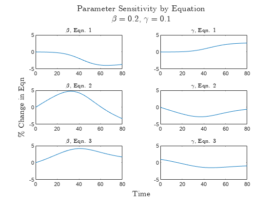
The results in the first row show that the values of $\beta$ and $\gamma$ affect the population of susceptible people more as time goes on in the simulation. $\beta$ works to decrease the population of susceptible people directly by increasing the number of infected people, while $\gamma$ acts on the susceptible group indirectly by controlling how quickly infected people recover from the disease versus continuing to infect others.

The results in the second row show that $\beta$ and $\gamma$ affect the population of infected people most in the middle of the simulation.

The results in the third row show that $\beta$ has the strongest effect on the population of recovered people, but the effect decreases from the middle to end of the simulation.

References

[1] "Compartmental Models in Epidemiology." Wikipedia, January 4, 2024. https://en.wikipedia.org/wiki/Compartmental_models_in_epidemiology.

[2] Hearne, J. W. “Sensitivity Analysis of Parameter Combinations.” Applied Mathematical Modelling 9, no. 2 (April 1985): pp. 106–8. https://doi.org/10.1016/0307-904X(85)90121-0.