Compressing Neural Networks Using Network Projection
By Antoni Woss, MathWorks
Deploying increasingly large and complex deep learning networks onto resource-constrained devices is a growing challenge facing many AI practitioners. This is because modern deep neural networks typically run on highly performing processors and GPUs and feature many millions of learnable parameters. Deploying these powerful deep learning models onto edge devices often requires compressing them to reduce size on disk, runtime memory, and inference times, while attempting to retain high accuracy and model expressivity.
There are numerous techniques for compressing deep learning networks—such as pruning and quantization—that can be used in tandem. This article introduces a new technique: network projection. This technique analyzes the covariance of neural excitations on layers of interest and reduces the number of learnable parameters by modifying layers to operate in a projective space. Although the operations of the layer take place in a typically lower rank projective space, the expressivity of the layer remains high as the width—i.e., the number of neural activations—remains unchanged when compared to the original network architecture. This can be used in place of or in addition to pruning and quantization.
Network Compression via Projection
Training a deep neural network amounts to determining a point in the corresponding high-dimensional space of learnable parameters that minimizes some specified loss function. The most common approaches to determining this optimal value are through gradient descent minimizations and variations thereof. To overcome a lack of knowledge of the underlying function that you seek to determine, deep network architectures with an abundance of learnable parameters are proposed to facilitate sufficient expressivity needed to find a suitable function. These can ultimately be vastly over-parameterized for the task at hand and necessarily result in a high degree of correlation between neurons in the network.
Network projection approaches the problem of compression by analyzing these neural correlations before carefully introducing projective operations that ultimately reduce the number of learnable parameters in the network, while retaining the important neural relations to preserve accuracy and expressivity.
Background
To set up the discussion, begin by defining a simple network, \( F: \mathbb{R}^{a_0} → \mathbb{R}^{a_N} \), as the composition of \( N \) functions: \[ F(x) = f_N (f_{N-1} (... f_{1} (x) ...)) \]
Here, \( f_i:\mathbb{R}^{a_{i−1}}→\mathbb{R}^{a_i} \) denotes the functional operation of layer \(i \), the dimension of the domain for \(f_i \) is \(a_{i−1} \in \mathbb{N} \) and \(x \in \mathbb{R}^{a_0} \) is some input tensor to the network. Note that \(a_i \) is written to denote the product of all dimensions of the tensor. For example, a convolutional neural network trained for an image classification task propagates images, \(x_{h,w,c} \in \mathbb{R}^{H×W×C} \), where \(H \) and \(W \) are the height and width of the image respectively and the number of color channels is \(C \).
A neuron is defined as an elementwise component of \(f_i \). More formally, there are \(a_i \) neurons on the \(i \)-th layer and for \(k=1,…,a_i \), a neuron is the scalar function, \( n^{(k)}_i(x):\mathbb{R}^{a_{i-1}}→\mathbb{R} \). For example, for a fully connected layer that takes three inputs to two outputs, there are two neurons that take a three-vector to a scalar (Figure 1).
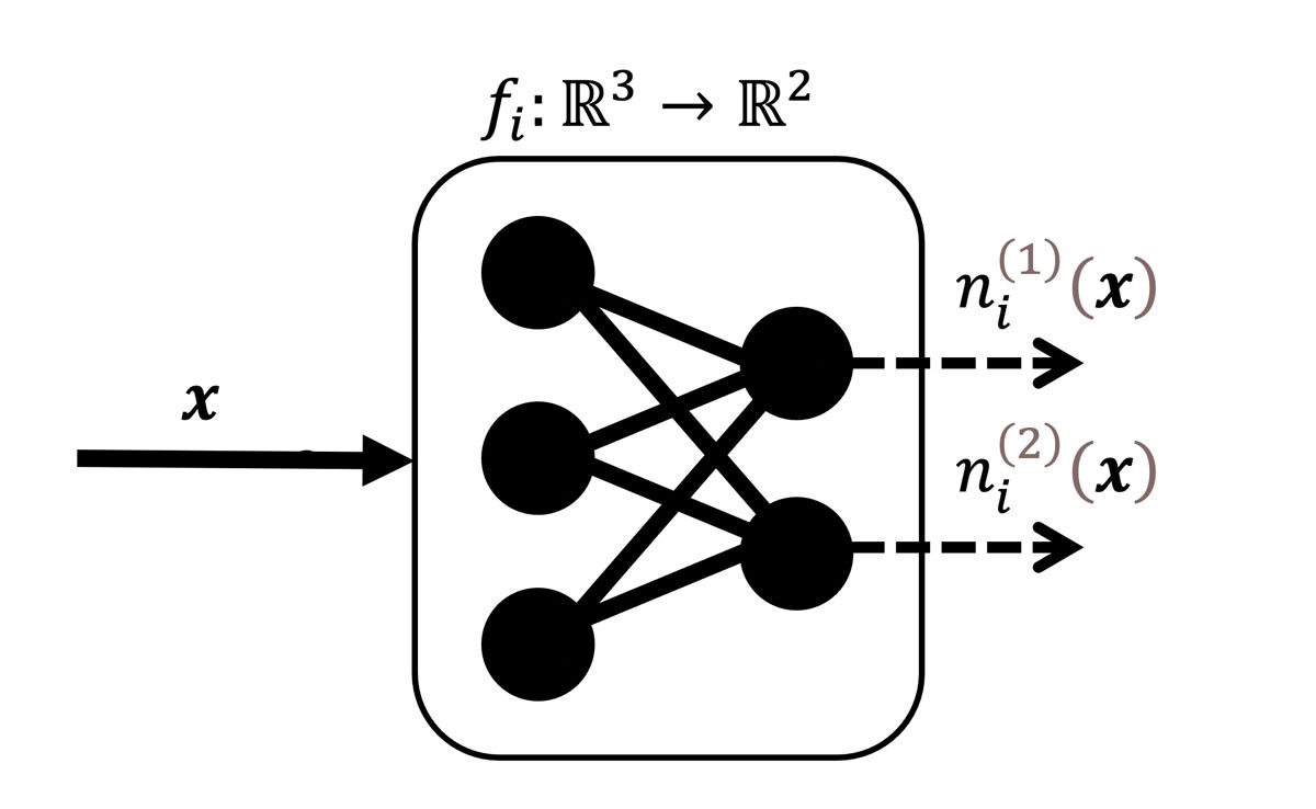
Figure 1. A toy example of a fully connected layer with two neurons.
Neural Covariance
As a deep learning network trains, learnable parameters move around the high-dimensional space in a correlated way, with a trajectory determined by choice of minimization routine, network initialization, and the training data. The neurons in the resulting trained network can therefore exhibit a high degree of correlation. You can measure the covariance between the neurons on each layer by stimulating the neurons with data representative of the true data distribution you train the network on, and then compute the neural covariance matrix with respect to these neural excitations.
To determine the neural covariance matrix for layer \(i\), first compute a set of neural excitations, \( \{ n^{(k)}(x_b) \, \vert \, k=1,…,a_i \,\,\)and \(\,\, \forall 𝒙_b \in X \} \), where \(X \) is representative of the distribution of training data, and \(b \) indexes the observation. It follows that the components of the neural covariance matrix are: \[ C_{pq}= \underset{b}cov (n^{(p)}(x_b),n^{(q)}(x_b)) \]
where \(p,q=1,…,a_i \) and the covariance is taken with respect to the observation index, \(b \). For example, for the fully connected layer in Figure 1, the covariance matrix would be a 2x2 matrix with the diagonal elements being the variance of the two neurons and the off-diagonal entry being the covariance between them.
The covariance matrix is positive semi-definite, symmetric, and has eigenvalues \(λ_p≥0 \) where \(p=1,…,a_i \). The corresponding eigenvectors, \(v_p \), form an orthonormal set and diagonalize the covariance matrix via conjugation with respect to this set. The eigenvectors and corresponding eigenvalues give the directions and magnitude of variance respectively. This means that small eigenvalues near zero correspond to linear combinations of neurons that carry near zero variance through this layer. On the contrary, eigenvectors with corresponding large eigenvalues denote linear combinations of neurons that propagate large variance. The linear combinations of neurons, defined by the eigenvectors, are referred to as eigenneurons.
This analysis of covariance motivates the construction of a projection operator, \(\mathbb{P} \), that projects the neurons into a subspace \(\mathbb{R}^{b_i}⊂\mathbb{R}^{a_i} \), with \( b_i ≤ a_i \), by eliminating contributions from eigenneurons that carry negligible variance. The projection operation can be expressed as the outer product of eigenvectors: \[ \mathbb{P}= \sum^{b_i}_{p=1}{v_p}{v^T_p} \]
Here, eigenvectors are ordered with respect to decreasing eigenvalues, \(λ_p≥λ_{p+1} \), and you can choose \(b_i \) depending on the amount of variance to retain. For example, if you want to retain an amount of explained variance (the cumulative variance sum), choose the smallest \(b_i \) such that: \[ 1−ϵ < \frac{ \sum^{b_i}_{p=1}λ_p}{\sum^{a_i}_{p=1}λ_p} \]
where \( 1−ϵ \) is the explained variance to retain. In the limit that \(b_i→a_i \), the projection operator tends to the identity matrix, \(\mathbb{P}→\mathbb{I} \), and the projection operation is trivial. Also, in the limit that \(ϵ→0 \), i.e., explained variance is 1, \(b_i→a_i \), and the projection operation again tends to the identity matrix. These limits show the connection to the original network.
The Projection Framework
The projection operation applied to the neurons of a layer defines a projected layer. More formally, the projection operation can be used to define a mapping from a layer to its projected equivalent, \(f^{\mathbb{P}}_i \), given by: \[ f^{\mathbb{P}}_i: \mathbb{R}^{a_{i−1}} → \mathbb{R}^{a_i} \] \[x\ ↦ \mathbb{P}_i{f}_i(\mathbb{P}_{i-1}x)\]
where the input and output neurons are projected. This mapping extends to the projection of a network. A projected network is the composition of projected layers: \[ F(x) = f^{\mathbb{P}}_N (f^{\mathbb{P}}_{N-1} (... f^{\mathbb{P}}_{1} (x) ...)) \]
Applying the projection operator layer-by-layer simply amounts to transforming the neurons in each layer to the corresponding eigenneurons, reducing the rank by eliminating low-variance eigenneurons, then transforming back into the original basis of neurons before feeding into the next layer (Figure 2).
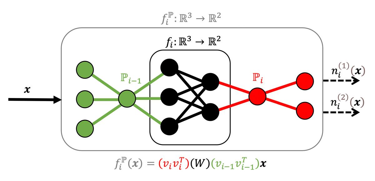
Figure 2. Projected fully connected layer based on Figure 1, with a rank-1 input and output projection operation. The layer operation is written explicitly in the figure, assuming for simplicity in this example that there is no bias term in the fully connected layer.
In this framework, different layers can be projected by varying amounts, depending on the rank of the layers input and output projection operators. Furthermore, any layer can be swapped for its projected equivalent without a need to change the downstream architecture, making this projective technique applicable to almost any network architecture, not just feedforward networks.
Compression
For many layers with learnable parameters—such as fully connected, convolution, and LSTM—the layer operations can be modified to absorb the projection operation into the learnable parameters. This ultimately reduces the number of learnable parameters on the projected layer with respect to the original, thus compressing the layer (Figure 3).
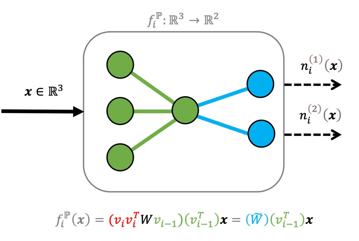
Figure 3. Projected fully connected layer. The layer operation is written under the figure and shows how the projected weight matrix, \(\widetilde W \), is given as the product of the original weight matrix, \(W \), and projection matrices.
For the fully connected layer in Figure 1 and the projected fully connected layer in Figure 3—assuming for simplicity that there is no bias term—each edge represents a learnable parameter, or an element in the weight matrix. For Figure 1, there are six learnable parameters in the weight matrix whereas the projected layer has five. This reduces the size of the layer, trading one large matrix multiplication for two smaller ones.
It is important to note that the distribution of the training data drives the construction of the projection operation, which, in turn, drives the decomposition of the weight matrices. This contrasts with simply taking a singular value decomposition of the weight matrices in the layers as the neural covariance matrix may favor a different subspace to that spanned by the SVD factors.
The precise implementation of projection depends on the layer itself. Furthermore, the number of neurons on each layer— \(a_i \)—is often extremely large. For example, the convolutional layers for a typical object detector network, such as YOLO v4, may have \(O(10^6) \) neurons, making it unfeasible to compute the neural covariance matrix. It is often desirable instead to consider covariances of carefully chosen operations that reduce this dimensionality: for example, average pooling in the spatial dimensions of a convolutional layer and examining the covariance in the channel dimension only. Each layer and use case necessitate consideration for the most appropriate covariance computation.
Fine-Tuning
Starting with a pretrained network, the projected network equivalent can be directly computed as outlined in the framework above. Although a high degree of data covariance is retained, the network may need fine-tuning as accuracy can drop following the compression. This could be a result of higher order nonlinear relations between neurons in the network needing to readjust given the linear transformation or a compounding effect if many layers are projected at once. The projected model provides a good initialization for fine-tuning by further retraining. The fine-tune retraining typically takes far fewer epochs for the accuracy to plateau and can largely recover, in many cases, the accuracy of the original network.
Examples and More
One illustration of where compression using projection has been successfully applied is in building a virtual sensor for battery state-of-charge (BSOC) estimation.
For a variety of reasons, it is not physically possible to build a deployable sensor to measure SOC directly. This is a common challenge for many systems across industries, not only for batteries. A tempting choice is to estimate SOC using an extended Kalman filter (EKF). An EKF can be extremely accurate, but it requires having a nonlinear mathematical model of a battery, which is not always available or feasible to create. A Kalman filter can also be computationally expensive and, if an initial state is wrong or of the model is not correct, it can produce inaccurate results.
An alternative is to develop a virtual sensor using an RNN network featuring LSTM layers. Such models have been shown to produce highly accurate results when trained on quality data, however, the models are often large in size and yield slow inference speeds. The LSTM layers in the network can be compressed using projection to reduce the overall network size and improve inference speed, while retaining high accuracy on the data set. A typical architecture for a projected LSTM network used for BSOC estimation is shown in Table 1.
| Name | Type | Activations | Learnable Properties | |
| 1 | sequenceinputSequence input with three dimensions |
Sequence Input | 3(C) x 1(B) x 1(T) | - |
| 2 | lstm_1Projected LSTM layer with 256 hidden units |
Projected LSTM | 256(C) x 1(B) x 1(T) | InputWeights 1024 x 3 Recurrent Weights 1024 x 11 Bias 1024 x 1 InputProjector 3 x 3 OutputProjector 256 x 11 |
| 3 | dropout_120% dropout |
Dropout | 256(C) x 1(B) x 1(T) | - |
| 4 | lstm_2Projected LSTM layer with 128 hidden units |
Projected LSTM | 128(C) x 1(B) x 1(T) | InputWeights 512 x 11 Recurrent Weights 512 x 8 Bias 512 x 1 InputProjector 256 x 11 OutputProjector 128 x 8 |
| 5 | dropout_220% dropout |
Dropout | 128(C) x 1(B) x 1(T) | - |
| 6 | fcOne fully connected layer |
Fully Connected | 1(C) x 1(B) x 1(T) | Weights 1 x 128 Bias 1 x 1 |
| 7 | layersigmoid |
Sigmoid | 1(C) x 1(B) x 1(T) | - |
| 8 | regressionoutputmean-squared-error with response ‘Response’ |
Regression Output | 1(C) x 1(B) x 1(T) | - |
Table 1. Analysis of a projected LSTM network architecture used in BSOC estimation.
Figure 4 shows a comparison of model accuracy (as a measure of RMSE), model size (as the number of learnable parameters), and inference speed (running as a MEX file in MATLAB), for this BSOC RNN network with an LSTM layer, before and after projection and fine-tuning.
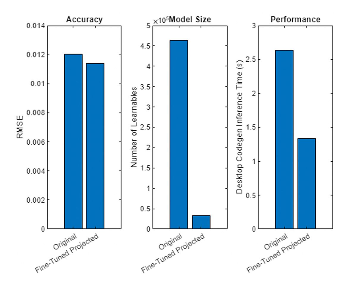
Figure 4. A comparison of accuracy, model size, and inference speed for a recurrent neural network with an LSTM layer, modeling battery state of charge, before and after projection with fine-tuning.
To project and compress networks of your own, try out the features available from MATLAB R2022b, compressNetworkUsingProjection and neuronPCA, by installing Deep Learning Toolbox™ together with the Deep Learning Toolbox Model Quantization Library.
Published 2023