quantiz
Produce quantization index and quantized output value
Syntax
Description
[
specifies index,quants] = quantiz(sig,partition,codebook)codebook, which prescribes a value for each partition in the
scalar quantization. codebook is a vector whose length must exceed the
length of partition by one. The function also returns
quants, which contains the scalar quantization of
sig and depends on the quantization levels and prescribed values in
the codebook.
Examples
Show how the quantiz function uses partition and codebook to map a real vector, samp, to a new vector, quantized, whose entries are either -1, 0.5, 2, or 3.
Generate sample data and specify partition and codebook vectors. Specify the partition vector by defining the distinct endpoints of the different intervals as the element values of the vector. Specify the codebook vector with an element value for each interval defined in the partition vector. The codebook vector must be one element longer than the partition vector.
samp = [-2.4, -1, 0, 0.2, 0.8, 1.2, 2,3, 3.5, 5];
partition = [0, 1, 3];
codebook = [-1, 0.5, 2, 3];
Quantize the data samples. Display the input sample data, the quantization index, and the corresponding quantized output value of the input data.
[index,quantized] = quantiz(samp,partition,codebook);
[samp; index; quantized]'
ans = 10×3

   -2.4000         0   -1.0000
   -1.0000         0   -1.0000
         0         0   -1.0000
    0.2000    1.0000    0.5000
    0.8000    1.0000    0.5000
    1.2000    2.0000    2.0000
    2.0000    2.0000    2.0000
    3.0000    2.0000    2.0000
    3.5000    3.0000    3.0000
    5.0000    3.0000    3.0000
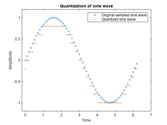
To illustrate the nature of scalar quantization, this example shows how to quantize a sine wave. Plot the original and quantized signals to contrast the x symbols that make up the sine curve with the dots that make up the quantized signal. The vertical coordinate of each dot is a value in the vector codebook.
Generate a sine wave sampled at times defined by t. Specify the partition input by defining the distinct endpoints of the different intervals as the element values of the vector. Specify the codebook input with an element value for each interval defined in the partition vector. The codebook vector must be one element longer than the partition vector.
t = [0:.1:2*pi];
sig = sin(t);
partition = [-1:.2:1];
codebook = [-1.2:.2:1];
Perform quantization on the sampled sine wave.
[index,quants] = quantiz(sig,partition,codebook);
Plot the quantized sine wave and the sampled sine wave.
plot(t,sig,'x',t,quants,'.')
title('Quantization of Sine Wave')
xlabel('Time')
ylabel('Amplitude')
legend('Original sampled sine wave','Quantized sine wave');
axis([-.2 7 -1.2 1.2])

Testing and selecting parameters for large signal sets with a fine quantization scheme can be tedious. One way to produce partition and codebook parameters easily is to optimize them according to a set of training data. The training data should be typical of the kinds of signals to be quantized.
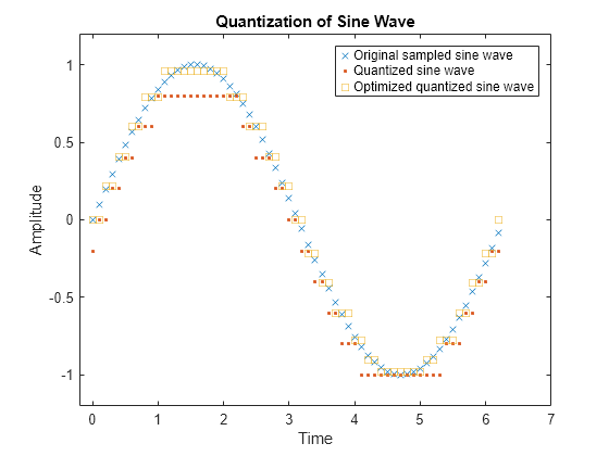
This example uses the lloyds function to optimize the partition and codebook according to the Lloyd algorithm. The code optimizes the partition and codebook for one period of a sinusoidal signal, starting from a rough initial guess. Then the example runs the quantiz function twice to generate quantized data by using the initial partition and codebook input values and by using the optimized partitionOpt and codebookOpt input values. The example also compares the distortion for the initial and the optimized quantization.
Define variables for a sine wave signal and initial quantization parameters. Optimize the partition and codebook by using the lloyds function.
t = 0:.1:2*pi;
sig = sin(t);
partition = -1:.2:1;
codebook = -1.2:.2:1;
[partitionOpt,codebookOpt] = lloyds(sig,codebook);
Generate quantized signals by using the initial and the optimized partition and codebook vectors. The quantiz function automatically computes the mean square distortion and returns it as the third output argument. Compare mean square distortions for quantization with the initial and optimized input arguments to see how less distortion occurs when using the optimized quantized values.
[index,quants,distor] = quantiz(sig,partition,codebook);
[indexOpt,quantOpt,distorOpt] = ...
    quantiz(sig,partitionOpt,codebookOpt);
[distor, distorOpt]
ans = 1×2
0.0148 0.0022
Plot the sampled sine wave, the quantized sine wave, and the optimized quantized sine wave.
plot(t,sig,'x',t,quants,'.',t,quantOpt,'s')
title('Quantization of Sine Wave')
xlabel('Time')
ylabel('Amplitude')
legend('Original sampled sine wave', ...
    'Quantized sine wave', ...
    'Optimized quantized sine wave');
axis([-.2 7 -1.2 1.2])

Input Arguments
Input signal, specified as a vector. This input specifies the sampled signal for this function to perform quantization.
Data Types: double
Distinct endpoints of different ranges, specified as a row vector. This input defines several contiguous, nonoverlapping ranges of values within the set of real numbers. The values present in this input must be strictly in ascending order. The length of this vector must be one less than the number of partition intervals.
Example: [0, 1, 3]
partitions the input row vector into the four sets {X:
X ≤ 0}, {X:
0 < X ≤ 1},
{X: 1 < X ≤
3}, and {X: 3 <
X}.
Data Types: double
Quantization value for each partition, specified as a row vector. This input
prescribes a common value for each partition in the scalar quantization. The length of
this vector must equal the number of partition intervals, that is, the length of this
vector must exceed the length of the partition input by one.
Data Types: double
Output Arguments
Quantization index of the input signal, returned as a nonnegative row vector. This
output determines on which partition interval, each input value is mapped. Each element
in index is one of the N integers in the range
[0, N–1].
If the partition input has length N,
index is a vector whose Kth entry is:
0ifsig(K) ≤partition(1)M if
partition(M) <sig(K) ≤partition(M+1)N if
partition(N) ≤sig(K)
Output of the quantizer, which contains the quantization values of the input signal,
returned as a row vector. The size of quants matches that of input
argument sig. When codebook is not specified
as an input argument, you can define the codebook values as a vector whose length must
exceed the length of the partition by one.
quants is calculated based on the codebook
and index inputs and is given by
quants(i) =
codebook(index(i) + 1), where
i is an integer in the range [1,
length(].sig)
Mean square distortion of the quantized signal, returned as a positive scalar. You
can reduce this distortion by choosing appropriate partition and codebook values. For
more information on optimizing partition and codebook values, see the lloyds function.
Version History
Introduced before R2006a
See Also
Functions
lloyds|dpcmenco|dpcmdeco|huffmanenco|huffmandeco|arithenco|arithdeco|compand
Topics
MATLAB Command
You clicked a link that corresponds to this MATLAB command:
Run the command by entering it in the MATLAB Command Window. Web browsers do not support MATLAB commands.
Select a Web Site
Choose a web site to get translated content where available and see local events and offers. Based on your location, we recommend that you select: .
You can also select a web site from the following list
How to Get Best Site Performance
Select the China site (in Chinese or English) for best site performance. Other MathWorks country sites are not optimized for visits from your location.
Americas
- América Latina (Español)
- Canada (English)
- United States (English)
Europe
- Belgium (English)
- Denmark (English)
- Deutschland (Deutsch)
- España (Español)
- Finland (English)
- France (Français)
- Ireland (English)
- Italia (Italiano)
- Luxembourg (English)
- Netherlands (English)
- Norway (English)
- Österreich (Deutsch)
- Portugal (English)
- Sweden (English)
- Switzerland
- United Kingdom (English)