Two-Degree-of-Freedom PID Controllers
Two-degree-of-freedom (2-DOF) PID controllers include setpoint weighting on the proportional and derivative terms. A 2-DOF PID controller is capable of fast disturbance rejection without significant increase of overshoot in setpoint tracking. 2-DOF PID controllers are also useful to mitigate the influence of changes in the reference signal on the control signal.
You can represent PID controllers using the specialized model objects
pid2 and pidstd2. This topic describes the
representation of 2-DOF PID controllers in MATLAB®. For information about automatic PID controller tuning, see PID Controller Tuning.
Continuous-Time 2-DOF PID Controller Representations
This illustration shows a typical control architecture using a 2-DOF PID controller.
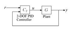
The relationship between the 2-DOF controller’s output (u) and its two inputs (r and y) can be represented in either parallel or standard form. The two forms differ in the parameters used to express the proportional, integral, and derivative actions of the controller, as expressed in the following table.
| Form | Formula |
|---|---|
Parallel (pid2
object) |
In this representation:
|
Standard (pidstd2
object) |
In this representation:
|
Use a controller form that is convenient for your application. For instance, if
you want to express the integrator and derivative actions in terms of time
constants, use standard form. For examples showing how to create parallel-form and
standard-form controllers, see the pid2 and pidstd2 reference pages,
respectively.
For information on representing PID Controllers in discrete time, see Discrete-Time Proportional-Integral-Derivative (PID) Controllers.
2-DOF Control Architectures
The 2-DOF PID controller is a two-input, one output controller of the form C2(s), as shown in the following figure. The transfer function from each input to the output is itself a PID controller.
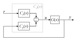
Each of the components Cr(s) and Cy(s) is a PID controller, with different weights on the proportional and derivative terms. For example, in continuous time, these components are given by:
You can access these components by converting the PID controller into a two-input,
one-output transfer function. For example, suppose that C2 is a
2-DOF PID controller, stored as a pid2 object.
C2tf = tf(C2);
Cr = C2tf(1);
Cy = C2tf(2);
Cr(s) is the transfer
function from the first input of C2 to the output. Similarly,
Cy(s) is the
transfer function from the second input of C2 to the
output.
Suppose that G is a dynamic system model, such as a zpk model, representing the plant.
Build the closed-loop transfer function from r to
y. Note that the
Cy(s) loop has
positive feedback, by the definition of
Cy(s).
T = Cr*feedback(G,Cy,+1)
Alternatively, use the connect command to build an
equivalent closed-loop system directly with the 2-DOF controller
C2. To do so, set the InputName and
OutputName properties of G and
C2.
G.InputName = 'u';
G.OutputName = 'y';
C2.Inputname = {'r','y'};
C2.OutputName = 'u';
T = connect(G,C2,'r','y');
There are other configurations in which you can decompose a 2-DOF PID controller
into SISO components. For particular choices of
C(s) and
X(s), each of the following configurations
is equivalent to the 2-DOF architecture with
C2(s). You can
obtain C(s) and
X(s) for each of these configurations
using the getComponents command.
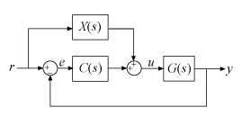
Feedforward
In the feedforward configuration, the 2-DOF PID controller is decomposed into a conventional SISO PID controller that takes the error signal as its input, and a feedforward controller.
For a continuous-time, parallel-form 2-DOF PID controller, the components are given by:
Access these components using getComponents.
[C,X] = getComponents(C2,'feedforward');
The following command constructs the closed-loop system from r to y for the feedforward configuration.
T = G*(C+X)*feedback(1,G*C);
Feedback
In the feedback configuration, the 2-DOF PID controller is decomposed into a conventional SISO PID controller and a feedback controller.
For a continuous-time, parallel-form 2-DOF PID controller, the components are given by:
Access these components using getComponents.
[C,X] = getComponents(C2,'feedback');
The following command constructs the closed-loop system from r to y for the feedback configuration.
T = G*C*feedback(1,G*(C+X));
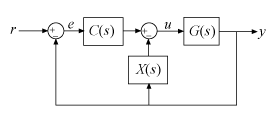
Filter
In the filter configuration, the 2-DOF PID controller is decomposed into a conventional SISO PID controller and a prefilter on the reference signal.
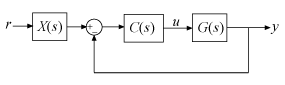
For a continuous-time, parallel-form 2-DOF PID controller, the components are given by:
The filter X(s) can also be expressed as the ratio: –[Cr(s)/Cy(s)].
The following command constructs the closed-loop system from r to y for the filter configuration.
T = X*feedback(G*C,1);
For an example illustrating the decomposition of a 2-DOF PID controller into these configurations, see Decompose a 2-DOF PID Controller into SISO Components.
The formulas shown above pertain to continuous-time, parallel-form
controllers. Standard-form controllers and controllers in discrete time can be
decomposed into analogous configurations. The getComponents command works on
all 2-DOF PID controller objects.
See Also
getComponents | pid2 | pidstd2 | pidtune | pidTuner