Compare Activation Layers
This example shows how to compare the accuracy of training networks with ReLU, leaky ReLU, ELU, and swish activation layers.
Training deep learning neural networks requires using nonlinear activation functions such as the ReLU and swish operations. Some activation layers can yield better training performance at the cost of extra computation time. When training a neural network, you can try using different activation layers to see if training improves.
This example shows how to compare the validation accuracy of training a SqueezeNet neural network when you use ReLU, leaky ReLU, ELU, or swish activation layers given a validation set of images.
Load Data
Download the Flowers data set.
url = "http://download.tensorflow.org/example_images/flower_photos.tgz";
downloadFolder = tempdir;
filename = fullfile(downloadFolder,"flower_dataset.tgz");

dataFolder = fullfile(downloadFolder,"flower_photos");
if ~exist(dataFolder,"dir")
    fprintf("Downloading Flowers data set (218 MB)... ")
    websave(filename,url);
    untar(filename,downloadFolder)
    fprintf("Done.\n")
end
Prepare Data for Training
Load the data as an image datastore using the imageDatastore function and specify the folder containing the image data.
imds = imageDatastore(dataFolder, ...
    IncludeSubfolders=true, ...
    LabelSource="foldernames");
View the number of classes of the training data.
numClasses = numel(categories(imds.Labels))
numClasses = 5
Divide the datastore so that each category in the training set has 80% of the images and the validation set has the remaining images from each label.
[imdsTrain,imdsValidation] = splitEachLabel(imds,0.80,"randomize");Specify augmentation options and create an augmented image datastore containing the training images.
Randomly reflect the images on the horizontal axis.
Randomly scale the images by up to 20%.
Randomly rotate the images by up to 45 degrees.
Randomly translate the images by up to 3 pixels.
Resize the images to the input size of the network (227-by-227).
imageAugmenter = imageDataAugmenter( ...
    RandXReflection=true, ...
    RandScale=[0.8 1.2], ...
    RandRotation=[-45,45], ...
    RandXTranslation=[-3 3], ...
    RandYTranslation=[-3 3]);

augimdsTrain = augmentedImageDatastore([227 227],imdsTrain,DataAugmentation=imageAugmenter);
Create an augmented image datastore for the validation data that resizes the images to the input size of the network. Do not apply any other image transformations to the validation data.
augimdsValidation = augmentedImageDatastore([227 227],imdsValidation);
Create Custom Plotting Function
When training multiple networks, to monitor the validation accuracy for each network on the same axis, you can use the OutputFcn training option and specify a function that updates a plot with the provided training information.
Create a function that takes the information structure provided by the training process and updates an animated line plot. The updatePlot function, listed in the Plotting Function section of the example, takes the information structure as input and updates the specified animated line.
Specify Training Options
Specify the training options:
Train using a mini-batch size of 128 for 60 epochs.
Shuffle the data each epoch.
Validate the neural network once per epoch using the held-out validation set.
miniBatchSize = 128;
numObservationsTrain = numel(imdsTrain.Files);
numIterationsPerEpoch = floor(numObservationsTrain / miniBatchSize);

options = trainingOptions("adam", ...
    MiniBatchSize=miniBatchSize, ...
    MaxEpochs=60, ...
    Shuffle="every-epoch", ...
    ValidationData=augimdsValidation, ...
    ValidationFrequency=numIterationsPerEpoch, ...
    Metrics="accuracy", ...
    Verbose=false);
Train Neural Networks
For each of the activation layer types—ReLU, leaky ReLU, ELU, and swish—train a SqueezeNet network.
Specify the types of activation layers.
activationLayerTypes = ["relu" "leaky-relu" "elu" "swish"];
Initialize the customized training progress plot by creating animated lines with colors specified by colororder function.
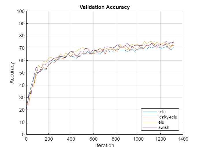
figure

colors = colororder;

for i = 1:numel(activationLayerTypes)
    line(i) = animatedline(Color=colors(i,:));
end

ylim([0 100])

legend(activationLayerTypes,Location="southeast");

xlabel("Iteration")
ylabel("Accuracy")
title("Validation Accuracy")
grid on
Loop over each of the activation layer types and train the neural network. For each activation layer type:
Create a function handle
activationLayerthat creates the activation layer.Create a new SqueezeNet network without weights and replace the activation layers (the ReLU layers) with layers of the activation layer type using the function handle
activationLayer.Replace the final convolution layer of the neural network with one specifying the number of classes of the input data.
Update the validation accuracy plot by setting the
OutputFcnproperty of the training options object to a function handle representing theupdatePlotfunction with the animated line corresponding to the activation layer type.Train and time the network using the
trainNetworkfunction.
for i = 1:numel(activationLayerTypes)
    activationLayerType = activationLayerTypes(i);

    % Determine activation layer type.
    switch activationLayerType
        case "relu"
            activationLayer = @reluLayer;
        case "leaky-relu"
            activationLayer = @leakyReluLayer;
        case "elu"
            activationLayer = @eluLayer;
        case "swish"
            activationLayer = @swishLayer;
    end

    % Create SqueezeNet with correct number of classes.
    net{i} = imagePretrainedNetwork("squeezenet",NumClasses=numClasses,Weights="none");

    % Replace activation layers.
    if activationLayerType ~= "relu"
        layers = net{i}.Layers;
        for j = 1:numel(layers)
            if isa(layers(j),"nnet.cnn.layer.ReLULayer")
                layerName = layers(j).Name;
                layer = activationLayer(Name=activationLayerType+"_new_"+j);
                net{i} = replaceLayer(net{i},layerName,layer);
            end
        end
    end

    % Specify custom plot function.
    options.OutputFcn = @(info) updatePlot(info,line(i));

    % Train the network.
    start = tic;
    [net{i},info{i}] = trainnet(augimdsTrain,net{i},"crossentropy",options);
    elapsed(i) = toc(start);
end
Visualize the training times in a bar chart.
figure
bar(categorical(activationLayerTypes),elapsed)
title("Training Time")
ylabel("Time (seconds)")
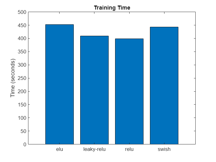
In this case, using the different activation layers yields similar final validation accuracies. When compared to the other activation layers, using ELU layers requires more computation time.
Plotting Function
The updatePlot function takes as input the information structure info and updates the validation plot specified by the animated line line. The function returns a logical value, stopFlag, which is always false. This ensures that the plotting function never causes training to stop early.
function stopFlag = updatePlot(info,line)

if ~isempty(info.ValidationAccuracy)
    addpoints(line,info.Iteration,info.ValidationAccuracy);
    drawnow limitrate
end
stopFlag = false;
end
See Also
trainnet | trainingOptions | dlnetwork | reluLayer | leakyReluLayer | swishLayer