Compare Deep Learning Models Using ROC Curves
This example shows how to use receiver operating characteristic (ROC) curves to compare the performance of deep learning models.
A ROC curve shows the true positive rate (TPR), or sensitivity, versus the false positive rate (FPR), or 1-specificity, for different thresholds of classification scores. The area under a ROC curve (AUC) corresponds to the integral of the curve (TPR values) with respect to FPR values from zero to one. The AUC provides an aggregate performance measure across all possible thresholds. The AUC values are in the range [0, 1], and larger AUC values indicate better classifier performance.
A perfect classifier always correctly assigns positive class observations to the positive class and has a TPR of 1 for all threshold values.
A random classifier returns random score values and has the same values for the FPR and TPR for all threshold values.

For a multiclass classification problem, the rocmetrics function formulates a set of one-versus-all binary classification problems with one binary problem for each class and finds a ROC curve for each class using the corresponding binary problem. Each binary problem assumes one class as positive and the rest as negative.
This example shows how to use ROC curves and AUC values to compare two methods of training a deep neural network for image classification.
Train a small network from scratch.
Adapt a pretrained GoogLeNet network for new data using transfer learning.
Load Data
Download and extract the Flowers [1] data set. The Flowers data set contains 3670 images of flowers belonging to five classes (daisy, dandelion, roses, sunflowers, and tulips).
url = "http://download.tensorflow.org/example_images/flower_photos.tgz";
downloadFolder = tempdir;
filename = fullfile(downloadFolder,"flower_dataset.tgz");

dataFolder = fullfile(downloadFolder,"flower_photos");
if ~exist(dataFolder,"dir")
    fprintf("Downloading Flowers data set (218 MB)... ")
    websave(filename,url);
    untar(filename,downloadFolder)
    fprintf("Done.\n")
end
numClasses = 5;
Create an image datastore containing the photos of the flowers.
imds = imageDatastore(dataFolder,IncludeSubfolders=true,LabelSource="foldernames");Partition the data into training, validation, and test sets. Set aside 20% of the data for validation and 20% of the data for testing using the splitEachLabel function.
[imdsTrain,imdsValidation,imdsTest] = splitEachLabel(imds,0.6,0.2,0.2,"randomize");Prepare Networks
Create two image classification models. For the first model, build and train a deep neural network from scratch. For the second model, adapt a pretrained GoogLeNet network for new data using transfer learning. This example requires the Deep Learning Toolbox™ Model for GoogLeNet Network support package. If this support package is not installed, then the googlenet function provides a download link. The GoogLeNet network requires images of size 224-by-224-by-3 pixels.
inputSize = [224 224 3];
Create New Network
Create a small network from scratch. Set the input size to match the input size of the GoogLeNet pretrained network. To reduce overfitting, include a dropout layer.
numFilters = 16;
filterSize = 3;
poolSize = 2;

smallNetLayers = [
    imageInputLayer(inputSize)

    convolution2dLayer(filterSize,numFilters,Padding="same")
    batchNormalizationLayer
    reluLayer
    maxPooling2dLayer(filterSize,Stride=2)

    convolution2dLayer(filterSize,2*numFilters,Padding="same")
    batchNormalizationLayer
    reluLayer
    maxPooling2dLayer(poolSize,Stride=2)

    convolution2dLayer(filterSize,4*numFilters,Padding="same")
    batchNormalizationLayer
    reluLayer
    maxPooling2dLayer(poolSize,Stride=2)

    dropoutLayer(0.8)

    fullyConnectedLayer(numClasses)
    softmaxLayer];
Prepare GoogLeNet Network
Adapt a pretrained GoogLeNet network for the new data.
Load a pretrained GoogLeNet network and the corresponding class names. This requires the Deep Learning Toolbox™ Model for GoogLeNet Network support package. If this support package is not installed, then the software provides a download link. For a list of all available networks, see Pretrained Deep Neural Networks. To return a neural network ready for retraining for the new data, also specify the number of classes.
googLeNet = imagePretrainedNetwork("googlenet",NumClasses=numClasses);Compare Networks
Compare the size of the networks using analyzeNetwork.
analyzeNetwork(googLeNet)
analyzeNetwork(smallNetLayers)
The small network has 17 layers and nearly 300,000 learnable parameters. The larger GoogleNet network has 144 layers and nearly 6 million learnable parameters. Although the pretrained network is larger, you do not need to train it for as long when you perform transfer learning. This reduction in training time is because the network has already learned features that you can use as a starting point for your new data.

Prepare Data
The networks require input images of size 224-by-224-by-3. To automatically resize the training images, use an augmented image datastore. Specify additional augmentation operations to perform on the training images: randomly flip the training images along the vertical axis and randomly scale them up to 50% horizontally and vertically. Data augmentation helps prevent the network from overfitting and memorizing the exact details of the training images.
augmenter = imageDataAugmenter(RandXReflection=true,RandScale=[0.5 1.5]);
augimdsTrain = augmentedImageDatastore(inputSize,imdsTrain,DataAugmentation=augmenter);
To automatically resize the validation images without performing further data augmentation, use an augmented image datastore without specifying any additional preprocessing operations.
augimdsValidation = augmentedImageDatastore(inputSize,imdsValidation);
Training Options
Train the small network for 100 epochs with an initial learning rate of 0.002.
optsSmallNet = trainingOptions("sgdm", ...
    MaxEpochs=100, ...
    InitialLearnRate=0.002, ...
    ValidationData=augimdsValidation, ...
    ValidationFrequency=150, ...
    Verbose=false, ...
    Plots="training-progress", ...
    Metrics="accuracy");
You do not need to train the pretrained network for as many epochs, so set the maximum number of epochs to 20. Previously, you increased the learning rate in the new learnable layer. To slow the learning in the earlier layers of the pretrained network, choose a small initial learning rate of 0.0001.
optsGoogLeNet = optsSmallNet;
optsGoogLeNet.MaxEpochs = 20;
optsGoogLeNet.InitialLearnRate = 0.0001;
Train Networks
Train the neural network using the trainnet function. For classification, use cross-entropy loss. By default, the trainnet function uses a GPU if one is available. Training on a GPU requires a Parallel Computing Toolbox™ license and a supported GPU device. For information on supported devices, see GPU Computing Requirements (Parallel Computing Toolbox). Otherwise, the trainnet function uses the CPU. To specify the execution environment, use the ExecutionEnvironment training option.
Despite being larger, the adapted GoogLeNet network converges quicker than the small network.
smallNet = trainnet(augimdsTrain,smallNetLayers,"crossentropy",optsSmallNet);
netGoogLeNet = trainnet(augimdsTrain,googLeNet,"crossentropy",optsGoogLeNet);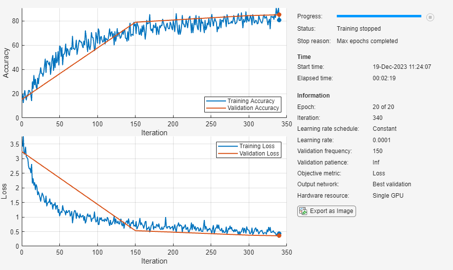
Compare Network Accuracy
Test the classification accuracy of the two networks by comparing the predictions on the test set with the true labels.
Prepare the test data.
augimdsTest = augmentedImageDatastore(inputSize,imdsTest);
TTest = imdsTest.Labels;
classNames = categories(TTest);
Classify the test images using the two networks. To make predictions with multiple observations, use the minibatchpredict function. To convert the prediction scores to labels, use the scores2label function. The minibatchpredict function automatically uses a GPU if one is available. Using a GPU requires a Parallel Computing Toolbox™ license and a supported GPU device. For information on supported devices, see GPU Computing Requirements (Parallel Computing Toolbox). Otherwise, the function uses the CPU.
scoresSmallNet = minibatchpredict(smallNet,augimdsTest);
YTestSmallNet = scores2label(scoresSmallNet,classNames);

scoresGoogLeNet = minibatchpredict(netGoogLeNet,augimdsTest);
YTestGoogLeNet = scores2label(scoresGoogLeNet,classNames);
Compare the accuracy of the two networks.
accSmallNet = sum(TTest == YTestSmallNet)/numel(TTest)
accSmallNet =
0.7061
accGoogLeNet = sum(TTest == YTestGoogLeNet)/numel(TTest)
accGoogLeNet =
0.8762
Plot confusion charts for each mode. For each class, the GoogLeNet network performs better than the smaller network. Both networks have the greatest difficulty in classifying images from the daisy and rose classes.
figure
tiledlayout(1,2)
nexttile
confusionchart(TTest,YTestSmallNet)
title("SmallNet")
nexttile
confusionchart(TTest,YTestGoogLeNet)
title("GoogLeNet")

Compare ROC Curves
You can use ROC curves to compare the performance of the two networks.
Create rocmetrics objects using the true labels in TTest and the classification scores from each of the trained networks. Specify the column order of the classification scores by extracting the class names from the output layers of each network.
rocSmallNet = rocmetrics(TTest,scoresSmallNet,classNames);
rocGoogLeNet = rocmetrics(TTest,scoresGoogLeNet,classNames);
rocSmallNet and rocGoogLeNet are rocmetrics objects that store the AUC values and performance metrics for each class in the AUC and Metrics properties. Plot the ROC curves for each class. You can click on any part of the ROC curve to see the threshold corresponding to the TPR and FPR values that you select.
The diagonal line indicates the performances of a random classifier. The smaller network performs the best for the sunflower and dandelion classes. However, across all five classes, the larger network performs better than the smaller network.
figure
tiledlayout(1,2,TileSpacing="compact")
nexttile
plot(rocSmallNet,ShowModelOperatingPoint=false)
legend(classNames)
title("ROC Curve: SmallNet")
nexttile
plot(rocGoogLeNet,ShowModelOperatingPoint=false)
legend(classNames)
title("ROC Curve: GoogLeNet")

Compare AUC Values
You can access the AUC value for each class using the rocmetrics object.
aucSmallNet = rocSmallNet.AUC;
aucGoogLeNet = rocGoogLeNet.AUC;
Compare the AUC values for each class. The AUC values provide an aggregate performance measure across all possible thresholds. The AUC values are in the range [0, 1], and larger AUC values indicate better classifier performance. For each class, the GoogLeNet network produces AUC values close to 1.
figure
bar([aucSmallNet; aucGoogLeNet]')
xticklabels(classNames)
legend(["SmallNet","GoogLeNet"],Location="southeast")
title("AUC")

Investigate Specific Class
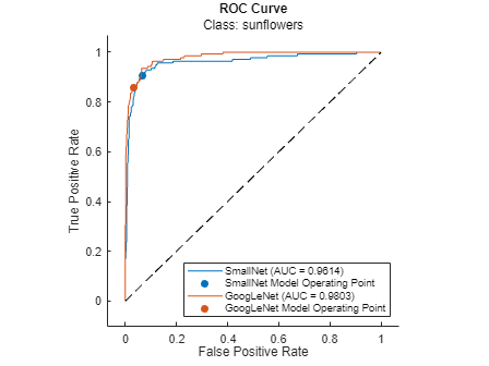
Investigate the ROC curves for the sunflowers class. By default, the plot function displays the class names and the AUC values in the legend. To include the model names in the legend instead of the class names, modify the DisplayName property of the ROCCurve object that the plot function returns. The model operating point represents the FPR and TPR corresponding to the typical threshold value. For the sunflower class, both models are performing well.
classToInvestigate = "sunflowers";

figure
c = cell(2,1);
g = cell(2,1);
[c{1},g{1}] = plot(rocSmallNet,ClassNames=classToInvestigate);
hold on
[c{2},g{2}] = plot(rocGoogLeNet,ClassNames=classToInvestigate);
modelNames = ["SmallNet","GoogLeNet"];
for i = 1:2
    c{i}.DisplayName = replace(c{i}.DisplayName, ...
        classToInvestigate,modelNames(i));
    g{i}(1).DisplayName = join([modelNames(i),"Model Operating Point"]);
end
title("ROC Curve","Class: " + classToInvestigate)
hold off
Compare Average ROC Curves
Find the average ROC curves. Specify AverageCurveType as "macro" to compute metrics for the average ROC curve using the macro-averaging method. Macro-averaging finds the average values of the FPR and TPR by averaging the values of the one-versus-all binary classification problems for each class. To learn more, see Average of Performance Metrics.
figure
averageType = "macro";
plot(rocSmallNet,AverageCurveType=averageType,ClassNames=[],ShowModelOperatingPoint=false)
hold on
plot(rocGoogLeNet,AverageCurveType=averageType,ClassNames=[],ShowModelOperatingPoint=false)
legend(["SmallNet (" + averageType + "-average)", ...
    "GoogLeNet (" + averageType + "-average)"])
hold off

References
[1] The TensorFlow Team. Flowers. http://download.tensorflow.org/example_images/flower_photos.tgz
See Also
rocmetrics | trainnet | trainingOptions | dlnetwork | confusionchart