Main Content

plot

Plot receiver operating characteristic (ROC) curves and other performance curves

Since R2022b

    Description

    example

    plot(rocObj) creates a receiver operating characteristic (ROC) curve, which is a plot of the true positive rate (TPR) versus the false positive rate (FPR), for each class in the ClassNames property of the rocmetrics object rocObj. The function marks the model operating point for each curve, and displays the value of the area under the ROC curve (AUC) and the class name for the curve in the legend.

    plot(ax,rocObj) creates the plot on the axes specified by ax instead of the current axes.

    example

    plot(___,Name=Value) specifies additional options using one or more name-value arguments in addition to any of the input argument combinations in the previous syntaxes. For example, AverageROCType="macro",ClassNames=[] computes the average performance metrics using the macro-averaging method and plots the average ROC curve only.

    example

    curveObj = plot(___) returns a ROCCurve object for each performance curve.

    [curveObj,graphicsObjs] = plot(___) also returns graphics objects for the model operating points and diagonal line.

    Examples

    collapse all

    Load a sample of predicted classification scores and true labels for a classification problem.

    load('flowersDataResponses.mat')

    trueLabels is the true labels for an image classification problem and scores is the softmax prediction scores. scores is an N-by-K array where N is the number of observations and K is the number of classes.

    trueLabels = flowersData.trueLabels;
    scores = flowersData.scores;

    Load the class names. The column order of scores follows the class order stored in classNames.

    classNames = flowersData.classNames;

    Create a rocmetrics object by using the true labels in trueLabels and the classification scores in scores. Specify the column order of scores using classNames.

    rocObj = rocmetrics(trueLabels,scores,classNames);

    rocObj is a rocmetrics object that stores the AUC values and performance metrics for each class in the AUC and Metrics properties. Display the AUC property.

    rocObj.AUC
    ans = 1x5 single row vector
    
        0.9781    0.9889    0.9728    0.9809    0.9732


    Plot the ROC curve for each class.

    plot(rocObj)

    Figure contains an axes object. The axes object with title ROC Curve, xlabel False Positive Rate, ylabel True Positive Rate contains 11 objects of type roccurve, scatter, line. These objects represent daisy (AUC = 0.9781), daisy Model Operating Point, dandelion (AUC = 0.9889), dandelion Model Operating Point, roses (AUC = 0.9728), roses Model Operating Point, sunflowers (AUC = 0.9809), sunflowers Model Operating Point, tulips (AUC = 0.9732), tulips Model Operating Point.

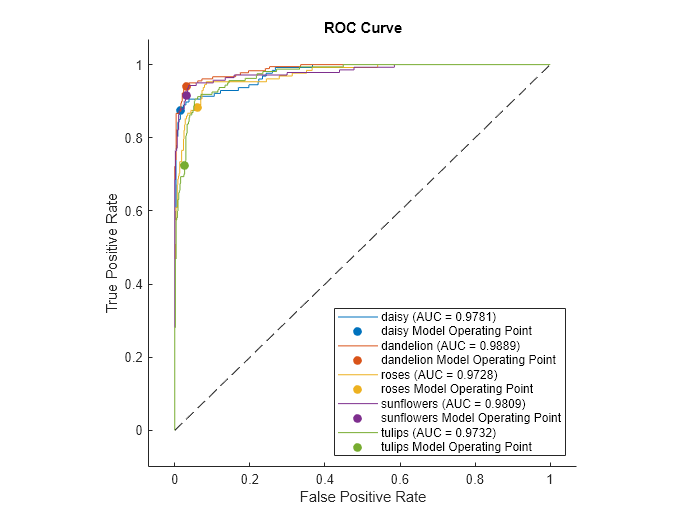
    The filled circle markers indicate the model operating points. The legend displays the class name and AUC value for each curve.

    Plot the macro average ROC curve.

    plot(rocObj,AverageROCType=["macro"],ClassNames=[])

    Figure contains an axes object. The axes object with title ROC Curve, xlabel False Positive Rate, ylabel True Positive Rate contains 2 objects of type roccurve, line. This object represents Macro-average (AUC = 0.9773).

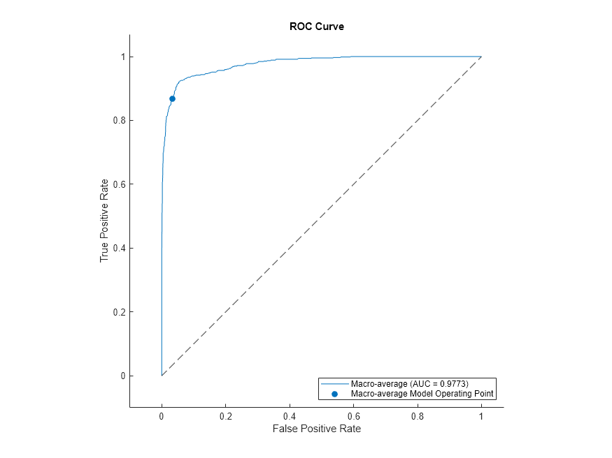
    Create a rocmetrics object and plot performance curves by using the plot function. Specify the XAxisMetric and YAxisMetric name-value arguments of the plot function to plot different types of performance curves other than the ROC curve. If you specify new metrics when you call the plot function, the function computes the new metrics and then uses them to plot the curve.

    Load a sample of true labels and the prediction scores for a classification problem. For this example, there are five classes: daisy, dandelion, roses, sunflowers, and tulips. The class names are stored in classNames. The scores are the softmax prediction scores generated using the predict function. scores is an N-by-K array where N is the number of observations and K is the number of classes. The column order of scores follows the class order stored in classNames.

    load('flowersDataResponses.mat')
    
    scores = flowersData.scores;
    trueLabels = flowersData.trueLabels;
    
    classNames = flowersData.classNames;

    Create a rocmetrics object. The rocmetrics function computes the FPR and TPR at different thresholds.

    rocObj = rocmetrics(trueLabels,scores,classNames);

    Plot the precision-recall curve for the first class. Specify the y-axis metric as precision (or positive predictive value) and the x-axis metric as recall (or true positive rate). The plot function computes the new metric values and plots the curve. Compute the area under the precision-recall curve using the trapezoidal method of the trapz function, and display the value in the legend.

    curveObj = plot(rocObj,ClassNames=classNames(1), ...
        YAxisMetric="PositivePredictiveValue",XAxisMetric="TruePositiveRate");
    xyData = rmmissing([curveObj.XData curveObj.YData]);
    auc = trapz(xyData(:,1),xyData(:,2));
    legend(join([string(classNames(1)) " (AUC = " string(auc) ")"],""), ...
        Location="southwest")
    title("Precision-Recall Curve")

    Figure contains an axes object. The axes object with title Precision-Recall Curve, xlabel True Positive Rate, ylabel Positive Predictive Value contains an object of type roccurve. This object represents daisy (AUC = 0.63331).

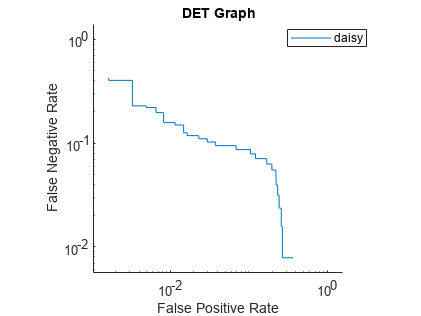
    Plot the detection error tradeoff (DET) graph for the first class. Specify the y-axis metric as the false negative rate and the x-axis metric as the false positive rate. Use a log scale for the x-axis and y-axis.

    f = figure;
    plot(rocObj,ClassNames=classNames(1), ...
        YAxisMetric="FalseNegativeRate",XAxisMetric="FalsePositiveRate")
    f.CurrentAxes.XScale = "log";
    f.CurrentAxes.YScale = "log";
    title("DET Graph")

    Figure contains an axes object. The axes object with title DET Graph, xlabel False Positive Rate, ylabel False Negative Rate contains an object of type roccurve. This object represents daisy.

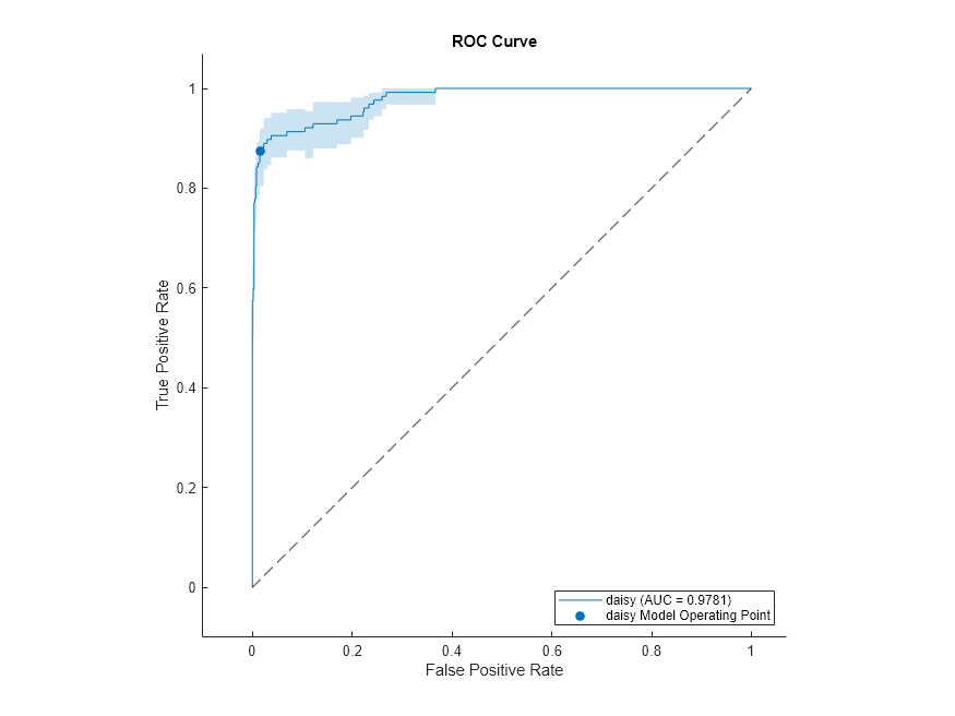
    Compute the confidence intervals for FPR and TPR for fixed threshold values by using bootstrap samples, and plot the confidence intervals for TPR on the ROC curve by using the plot function. This examples requires Statistics and Machine Learning Toolbox™.

    Load a sample of true labels and the prediction scores for a classification problem. For this example, there are five classes: daisy, dandelion, roses, sunflowers, and tulips. The class names are stored in classNames. The scores are the softmax prediction scores generated using the predict function. scores is an N-by-K array where N is the number of observations and K is the number of classes. The column order of scores follows the class order stored in classNames.

    load('flowersDataResponses.mat')
    
    scores = flowersData.scores;
    trueLabels = flowersData.trueLabels;
    
    classNames = flowersData.classNames;

    Create a rocmetrics object by using the true labels in trueLabels and the classification scores in scores. Specify the column order of scores using classNames. Specify NumBootstraps as 100 to use 100 bootstrap samples to compute the confidence intervals.

    rocObj = rocmetrics(trueLabels,scores,classNames,NumBootstraps=100);

    Plot the ROC curve and the confidence intervals for TPR. Specify ShowConfidenceIntervals=true to show the confidence intervals.

    plot(rocObj,ShowConfidenceIntervals=true)

    Figure contains an axes object. The axes object with title ROC Curve, xlabel False Positive Rate, ylabel True Positive Rate contains 11 objects of type roccurve, scatter, line. These objects represent daisy (AUC = 0.9781), daisy Model Operating Point, dandelion (AUC = 0.9889), dandelion Model Operating Point, roses (AUC = 0.9728), roses Model Operating Point, sunflowers (AUC = 0.9809), sunflowers Model Operating Point, tulips (AUC = 0.9732), tulips Model Operating Point.

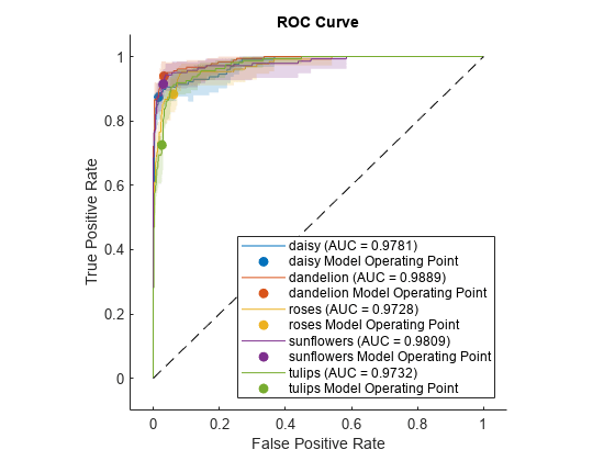
    The shaded area around each curve indicates the confidence intervals. rocmetrics computes the ROC curves using the scores. The confidence intervals represent the estimates of uncertainty for the curve.

    Specify one class to plot by using the ClassNames name-value argument.

    plot(rocObj,ShowConfidenceIntervals=true,ClassNames="daisy")

    Figure contains an axes object. The axes object with title ROC Curve, xlabel False Positive Rate, ylabel True Positive Rate contains 3 objects of type roccurve, scatter, line. These objects represent daisy (AUC = 0.9781), daisy Model Operating Point.

    Input Arguments

    collapse all

    Object evaluating classification performance, specified as a rocmetrics object.

    Target axes, specified as an Axes object.

    If you do not specify the axes and the current axes are Cartesian, then plot uses the current axes (gca). For more information on creating an Axes object, see axes and gca.

    Name-Value Arguments

    Specify optional pairs of arguments as Name1=Value1,...,NameN=ValueN, where Name is the argument name and Value is the corresponding value. Name-value arguments must appear after other arguments, but the order of the pairs does not matter.

    Example: YAxisMetric="PositivePredictiveValue",XAxisMetric="TruePositiveRate" plots the precision (positive predictive value) versus the recall (true positive rate), which represents a precision-recall curve.

    Method for averaging ROC curves, specified as "none", "micro", "macro", "weighted", a string array of method names, or a cell array of method names.

    • If you specify "none" (default), the plot function does not create the average ROC curve. The AverageROCType value must be "none" if plot creates performance curves other than a ROC curve.

    • If you specify multiple methods as a string array or a cell array of character vectors, then the plot function plots multiple average ROC curves using the specified methods.

    • If you specify one or more averaging methods and specify ClassNames=[], then the plot function plots only the average ROC curves.

    plot computes the averages of performance metrics for a multiclass classification problem, and plots the average ROC curves using these methods:

    • "micro" (micro-averaging) — plot finds the average performance metrics by treating all one-versus-all binary classification problems as one binary classification problem. The function computes the confusion matrix components for the combined binary classification problem, and then computes the average FPR and TPR using the values of the confusion matrix.

    • "macro" (macro-averaging) — plot computes the average values for FPR and TPR by averaging the values of all one-versus-all binary classification problems.

    • "weighted" (weighted macro-averaging) — plot computes the weighted average values for FPR and TPR using the macro-averaging method and using the prior class probabilities (the Prior property of rocObj) as weights.

    The algorithm type determines the length of the vectors in the XData, YData, and Thresholds properties of a ROCCurve object, returned by plot, for the average ROC curve. For more details, see Average of Performance Metrics.

    Example: AverageROCType="macro"

    Example: AverageROCType=["micro","macro"]

    Data Types: char | string

    Class labels to plot, specified as a categorical, character, or string array, logical or numeric vector, or cell array of character vectors. The values and data types in ClassNames must match those of the class names in the ClassNames property of rocObj. (The software treats character or string arrays as cell arrays of character vectors.)

    • If you specify multiple class labels, the plot function plots a ROC curve for each class.

    • If you specify ClassNames=[] and specify one or more averaging methods using AverageROCType, then the plot function plots only the average ROC curves.

    Example: ClassNames=["red","blue"]

    Data Types: single | double | logical | char | string | cell | categorical

    Flag to show the confidence intervals of the y-axis metric (YAxisMetric), specified as logical 0 (false) or 1 (true).

    The ShowConfidenceIntervals value can be true only if the Metrics property of rocObj contains the confidence intervals for the y-axis metric.

    Example: ShowConfidenceIntervals=true

    Using confidence intervals requires Statistics and Machine Learning Toolbox™.

    Data Types: logical

    Flag to show the diagonal line that extends from [0,0] to [1,1], specified as logical 1 (true) or 0 (false).

    The default value is true if you plot a ROC curve or an average ROC curve, and false otherwise.

    In the ROC curve plot, the diagonal line represents a random classifier, and the line passing through [0,0], [0,1], and [1,1] represents a perfect classifier.

    Example: ShowDiagonalLine=false

    Data Types: logical

    Flag to show the model operating point, specified as logical 1 (true) or 0 (false).

    The default value is true for a ROC curve, and false for an average ROC curve. The ShowModelOperatingPoint value must be false for performance curves other than ROC.

    Example: ShowModelOperatingPoint=false

    Data Types: logical

    Metric for the x-axis, specified as a character vector or string scalar of the built-in metric name or a custom metric name, or a function handle (@metricName).

    • Built-in metrics — Specify one of the following built-in metric names by using a character vector or string scalar.

      NameDescription
      "TruePositives" or "tp"Number of true positives (TP)
      "FalseNegatives" or "fn"Number of false negatives (FN)
      "FalsePositives" or "fp"Number of false positives (FP)
      "TrueNegatives" or "tn"Number of true negatives (TN)
      "SumOfTrueAndFalsePositives" or "tp+fp"Sum of TP and FP
      "RateOfPositivePredictions" or "rpp"Rate of positive predictions (RPP), (TP+FP)/(TP+FN+FP+TN)
      "RateOfNegativePredictions" or "rnp"Rate of negative predictions (RNP), (TN+FN)/(TP+FN+FP+TN)
      "Accuracy" or "accu"Accuracy, (TP+TN)/(TP+FN+FP+TN)
      "TruePositiveRate" or "tpr"True positive rate (TPR), also known as recall or sensitivity, TP/(TP+FN)
      "FalseNegativeRate", "fnr", or "miss"False negative rate (FNR), or miss rate, FN/(TP+FN)
      "FalsePositiveRate" or "fpr"False positive rate (FPR), also known as fallout or 1-specificity, FP/(TN+FP)
      "TrueNegativeRate", "tnr", or "spec"True negative rate (TNR), or specificity, TN/(TN+FP)
      "PositivePredictiveValue", "ppv", or "prec"Positive predictive value (PPV), or precision, TP/(TP+FP)
      "NegativePredictiveValue" or "npv"Negative predictive value (NPV), TN/(TN+FN)
      "ExpectedCost" or "ecost"

      Expected cost, (TP*cost(P|P)+FN*cost(N|P)+FP*cost(P|N)+TN*cost(N|N))/(TP+FN+FP+TN), where cost is a 2-by-2 misclassification cost matrix containing [0,cost(N|P);cost(P|N),0]. cost(N|P) is the cost of misclassifying a positive class (P) as a negative class (N), and cost(P|N) is the cost of misclassifying a negative class as a positive class.

      The software converts the K-by-K matrix specified by the Cost name-value argument of rocmetrics to a 2-by-2 matrix for each one-versus-all binary problem. For details, see Misclassification Cost Matrix.

      The software computes the scale vector using the prior class probabilities (Prior) and the number of classes in Labels, and then scales the performance metrics according to this scale vector. For details, see Performance Metrics.

    • Custom metric stored in the Metrics property — Specify the name of a custom metric stored in the Metrics property of the input object rocObj. The rocmetrics function names a custom metric "CustomMetricN", where N is the number that refers to the custom metric. For example, specify XAxisMetric="CustomMetric1" to use the first custom metric in Metrics as a metric for the x-axis.

    • Custom metric — Specify a new custom metric by using a function handle. A custom function that returns a performance metric must have this form:

      metric = customMetric(C,scale,cost)

      • The output argument metric is a scalar value.

      • A custom metric is a function of the confusion matrix (C), scale vector (scale), and cost matrix (cost). The software finds these input values for each one-versus-all binary problem. For details, see Performance Metrics.

        • C is a 2-by-2 confusion matrix consisting of [TP,FN;FP,TN].

        • scale is a 2-by-1 scale vector.

        • cost is a 2-by-2 misclassification cost matrix.

      The plot function names a custom metric "Custom Metric" for the axis label.

      The software does not support cross-validation for a custom metric. Instead, you can specify to use bootstrap when you create a rocmetrics object.

    If you specify a new metric instead of one in the Metrics property of the input object rocObj, the plot function computes and plots the metric values. If you compute confidence intervals when you create rocObj, the plot function also computes confidence intervals for the new metric.

    The plot function ignores NaNs in the performance metric values. Note that the positive predictive value (PPV) is NaN for the reject-all threshold for which TP = FP = 0, and the negative predictive value (NPV) is NaN for the accept-all threshold for which TN = FN = 0. For more details, see Thresholds, Fixed Metric, and Fixed Metric Values.

    Example: XAxisMetric="FalseNegativeRate"

    Data Types: char | string | function_handle

    Metric for the y-axis, specified as a character vector or string scalar of the built-in metric name or custom metric name, or a function handle (@metricName). For details, see XAxisMetric.

    Example: YAxisMetric="FalseNegativeRate"

    Data Types: char | string | function_handle

    Output Arguments

    collapse all

    Object for the performance curve, returned as a ROCCurve object or an array of ROCCurve objects. plot returns a ROCCurve object for each performance curve.

    Use curveObj to query and modify properties of the plot after creating it. For a list of properties, see ROCCurve Properties.

    Graphics objects for the model operating points and diagonal line, returned as a graphics array containing Scatter and Line objects.

    graphicsObjs contains a Scatter object for each model operating point (if ShowModelOperatingPoint=true) and a Line object for the diagonal line (if ShowDiagonalLine=true). Use graphicsObjs to query and modify properties of the model operating points and diagonal line after creating the plot. For a list of properties, see Scatter Properties and Line Properties.

    More About

    collapse all

    Receiver Operating Characteristic (ROC) Curve

    A ROC curve shows the true positive rate versus the false positive rate for different thresholds of classification scores.

    The true positive rate and the false positive rate are defined as follows:

    • True positive rate (TPR), also known as recall or sensitivity — TP/(TP+FN), where TP is the number of true positives and FN is the number of false negatives

    • False positive rate (FPR), also known as fallout or 1-specificity — FP/(TN+FP), where FP is the number of false positives and TN is the number of true negatives

    Each point on a ROC curve corresponds to a pair of TPR and FPR values for a specific threshold value. You can find different pairs of TPR and FPR values by varying the threshold value, and then create a ROC curve using the pairs. For each class, rocmetrics uses all distinct adjusted score values as threshold values to create a ROC curve.

    For a multiclass classification problem, rocmetrics formulates a set of one-versus-all binary classification problems to have one binary problem for each class, and finds a ROC curve for each class using the corresponding binary problem. Each binary problem assumes one class as positive and the rest as negative.

    For a binary classification problem, if you specify the classification scores as a matrix, rocmetrics formulates two one-versus-all binary classification problems. Each of these problems treats one class as a positive class and the other class as a negative class, and rocmetrics finds two ROC curves. Use one of the curves to evaluate the binary classification problem.

    For more details, see ROC Curve and Performance Metrics.

    Area Under ROC Curve (AUC)

    The area under a ROC curve (AUC) corresponds to the integral of a ROC curve (TPR values) with respect to FPR from FPR = 0 to FPR = 1.

    The AUC provides an aggregate performance measure across all possible thresholds. The AUC values are in the range 0 to 1, and larger AUC values indicate better classifier performance.

    One-Versus-All (OVA) Coding Design

    The one-versus-all (OVA) coding design reduces a multiclass classification problem to a set of binary classification problems. In this coding design, each binary classification treats one class as positive and the rest of the classes as negative. rocmetrics uses the OVA coding design for multiclass classification and evaluates the performance on each class by using the binary classification that the class is positive.

    For example, the OVA coding design for three classes formulates three binary classifications:

    Binary 1Binary 2Binary 3Class 1111Class 2111Class 3111

    Each row corresponds to a class, and each column corresponds to a binary classification problem. The first binary classification assumes that class 1 is a positive class and the rest of the classes are negative. rocmetrics evaluates the performance on the first class by using the first binary classification problem.

    Algorithms

    collapse all

    Adjusted Scores for Multiclass Classification Problem

    For each class, rocmetrics adjusts the classification scores (input argument Scores of rocmetrics) relative to the scores for the rest of the classes if you specify Scores as a matrix. Specifically, the adjusted score for a class given an observation is the difference between the score for the class and the maximum value of the scores for the rest of the classes.

    For example, if you have [s1,s2,s3] in a row of Scores for a classification problem with three classes, the adjusted score values are [s1-max(s2,s3),s2-max(s1,s3),s3-max(s1,s2)].

    rocmetrics computes the performance metrics using the adjusted score values for each class.

    For a binary classification problem, you can specify Scores as a two-column matrix or a column vector. Using a two-column matrix is a simpler option because the predict function of a classification object returns classification scores as a matrix, which you can pass to rocmetrics. If you pass scores in a two-column matrix, rocmetrics adjusts scores in the same way that it adjusts scores for multiclass classification, and it computes performance metrics for both classes. You can use the metric values for one of the two classes to evaluate the binary classification problem. The metric values for a class returned by rocmetrics when you pass a two-column matrix are equivalent to the metric values returned by rocmetrics when you specify classification scores for the class as a column vector.

    References

    [1] Sebastiani, Fabrizio. "Machine Learning in Automated Text Categorization." ACM Computing Surveys 34, no. 1 (March 2002): 1–47.

    Version History

    Introduced in R2022b