Interpret Deep Network Predictions on Numeric Feature Data Using LIME
This example shows how to use the locally interpretable model-agnostic explanations (LIME) technique to understand the predictions of a deep neural network classifying numeric feature data. You can use the LIME technique to understand which predictors are most important to the classification decision of a network.
In this example, you interpret a feature data classification network using LIME. For a specified query observation, LIME generates a synthetic data set whose statistics for each feature match the real data set. This synthetic data set is passed through the deep neural network to obtain a classification, and a simple, interpretable model is fitted. This simple model can be used to understand the importance of the top few features to the classification decision of the network. In training this interpretable model, synthetic observations are weighted by their distance from the query observation, so the explanation is "local" to that observation.
This example uses lime (Statistics and Machine Learning Toolbox) and fit (Statistics and Machine Learning Toolbox) to generate a synthetic data set and fit a simple interpretable model to the synthetic data set. To understand the predictions of a trained image classification neural network, use imageLIME. For more information, see Understand Network Predictions Using LIME.
Load Data
Load the Fisher iris data set. This data contains 150 observations with four input features representing the parameters of the plant and one categorical response representing the plant species. Each observation is classified as one of the three species: setosa, versicolor, or virginica. Each observation has four measurements: sepal width, sepal length, petal width, and petal length.
filename = fullfile(toolboxdir('stats'),'statsdata','fisheriris.mat');
load(filename)
Convert the numeric data to a table.
features = ["Sepal length","Sepal width","Petal length","Petal width"];

predictors = array2table(meas,"VariableNames",features);
trueLabels = array2table(categorical(species),"VariableNames","Response");
Create a table of training data whose final column is the response.
data = [predictors trueLabels];
Calculate the number of observations, features, and classes.
numObservations = size(predictors,1);
numFeatures = size(predictors,2);
classNames = categories(data{:,5});
numClasses = length(classNames);
Split Data into Training, Validation, and Test Sets
Partition the data set into training, validation, and test sets. Set aside 15% of the data for validation and 15% for testing.
Determine the number of observations for each partition. Set the random seed to make the data splitting and CPU training reproducible.
rng('default');
numObservationsTrain = floor(0.7*numObservations);
numObservationsValidation = floor(0.15*numObservations);
Create an array of random indices corresponding to the observations and partition it using the partition sizes.
idx = randperm(numObservations);
idxTrain = idx(1:numObservationsTrain);
idxValidation = idx(numObservationsTrain + 1:numObservationsTrain + numObservationsValidation);
idxTest = idx(numObservationsTrain + numObservationsValidation + 1:end);
Partition the table of data into training, validation, and testing partitions using the indices.
dataTrain = data(idxTrain,:);
dataVal = data(idxValidation,:);
dataTest = data(idxTest,:);
Define Network Architecture
Create a simple multi-layer perceptron, with a single hidden layer with five neurons and ReLU activations. The feature input layer accepts data containing numeric scalars representing features, such as the Fisher iris data set.
numHiddenUnits = 5;
layers = [
    featureInputLayer(numFeatures)
    fullyConnectedLayer(numHiddenUnits)
    reluLayer
    fullyConnectedLayer(numClasses)
    softmaxLayer];
Define Training Options and Train Network
Train the network using stochastic gradient descent with momentum (SGDM). Set the maximum number of epochs to 30 and use a mini-batch size of 15, as the training data does not contain many observations.
opts = trainingOptions("sgdm", ...
    MaxEpochs=30, ...
    MiniBatchSize=15, ...
    Shuffle="every-epoch", ...
    ValidationData=dataVal, ...
    Metrics="accuracy",...
    ExecutionEnvironment="cpu");
Train the neural network using the trainnet function. For classification, use cross-entropy loss.
net = trainnet(dataTrain,layers,"crossentropy",opts); Iteration Epoch TimeElapsed LearnRate TrainingLoss ValidationLoss TrainingAccuracy ValidationAccuracy
_________ _____ ___________ _________ ____________ ______________ ________________ __________________
0 0 00:00:10 0.01 1.4077 31.818
1 1 00:00:11 0.01 1.1628 46.667
50 8 00:00:13 0.01 0.50707 0.36361 86.667 90.909
100 15 00:00:13 0.01 0.19781 0.25353 86.667 90.909
150 22 00:00:13 0.01 0.26973 0.19193 86.667 95.455
200 29 00:00:14 0.01 0.20914 0.18269 86.667 90.909
210 30 00:00:14 0.01 0.3616 0.15335 73.333 95.455
Training stopped: Max epochs completed
Assess Network Performance
Classify observations from the test set using the trained network. To make predictions with multiple observations, use the minibatchpredict function. To convert the prediction scores to labels, use the scores2label function. The minibatchpredict function automatically uses a GPU if one is available. Using a GPU requires a Parallel Computing Toolbox™ license and a supported GPU device. For information on supported devices, see GPU Computing Requirements (Parallel Computing Toolbox). Otherwise, the function uses the CPU.
scores = minibatchpredict(net,dataTest(:,1:4));
predictedLabels = scores2label(scores,classNames);
trueLabels = dataTest{:,end};
Visualize the results using a confusion matrix.
figure
confusionchart(trueLabels,predictedLabels)

The network successfully uses the four plant features to predict the species of the test observations.
Understand How Different Predictors Are Important to Different Classes
Use LIME to understand the importance of each predictor to the classification decisions of the network.
Investigate the two most important predictors for each observation.
numImportantPredictors = 2;
Use lime to create a synthetic data set whose statistics for each feature match the real data set. Create a lime object using a deep learning model blackbox and the predictor data contained in predictors. Use a low 'KernelWidth' value so lime uses weights that are focused on the samples near the query point.
blackbox = @(x)scores2label(minibatchpredict(net,x),classNames);
explainer = lime(blackbox,predictors,'Type','classification','KernelWidth',0.1);
You can use the LIME explainer to understand the most important features to the deep neural network. The function estimates the importance of a feature by using a simple linear model that approximates the neural network in the vicinity of a query observation.
Find the indices of the first two observations in the test data corresponding to the setosa class.
trueLabelsTest = dataTest{:,end};
label = "setosa";
idxSetosa = find(trueLabelsTest == label,2);
Use the fit function to fit a simple linear model to the first two observations from the specified class.
explainerObs1 = fit(explainer,dataTest(idxSetosa(1),1:4),numImportantPredictors);
explainerObs2 = fit(explainer,dataTest(idxSetosa(2),1:4),numImportantPredictors);
Plot the results.
figure
subplot(2,1,1)
plot(explainerObs1);
subplot(2,1,2)
plot(explainerObs2);
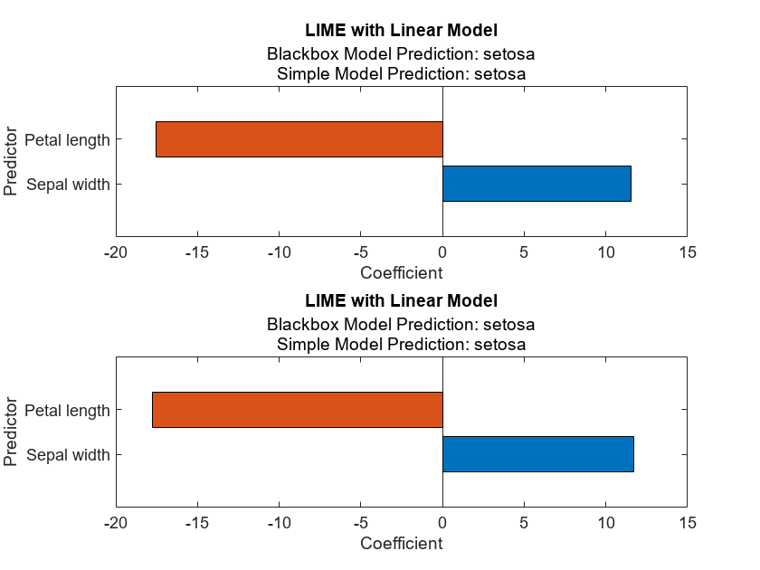
For the setosa class, the most important predictors are a low petal length value and a high sepal width value.
Perform the same analysis for class versicolor.
label = "versicolor";
idxVersicolor = find(trueLabelsTest == label,2);

explainerObs1 = fit(explainer,dataTest(idxVersicolor(1),1:4),numImportantPredictors);
explainerObs2 = fit(explainer,dataTest(idxVersicolor(2),1:4),numImportantPredictors);

figure
subplot(2,1,1)
plot(explainerObs1);
subplot(2,1,2)
plot(explainerObs2);
For the versicolor class, a high petal length value is important.
Finally, consider the virginica class.
label = "virginica";
idxVirginica = find(trueLabelsTest == label,2);

explainerObs1 = fit(explainer,dataTest(idxVirginica(1),1:4),numImportantPredictors);
explainerObs2 = fit(explainer,dataTest(idxVirginica(2),1:4),numImportantPredictors);

figure
subplot(2,1,1)
plot(explainerObs1);
subplot(2,1,2)
plot(explainerObs2);
For the virginica class, a high petal length value and a low sepal width value is important.
Validate LIME Hypothesis
The LIME plots suggest that a high petal length value is associated with the versicolor and virginica classes and a low petal length value is associated with the setosa class. You can investigate the results further by exploring the data.
Plot the petal length of each image in the data set.
setosaIdx = ismember(data{:,end},"setosa");
versicolorIdx = ismember(data{:,end},"versicolor");
virginicaIdx = ismember(data{:,end},"virginica");

figure
hold on
plot(data{setosaIdx,"Petal length"},'.')
plot(data{versicolorIdx,"Petal length"},'.')
plot(data{virginicaIdx,"Petal length"},'.')
hold off

xlabel("Observation number")
ylabel("Petal length")
legend(["setosa","versicolor","virginica"])
The setosa class has much lower petal length values than the other classes, matching the results produced from the lime model.
See Also
fit (Statistics and Machine Learning Toolbox) | lime (Statistics and Machine Learning Toolbox) | trainnet | trainingOptions | dlnetwork | testnet | minibatchpredict | scores2label | featureInputLayer | imageLIME