Deep Learning Visualization Methods
Deep learning networks are often described as "black boxes" because the reason that a network makes a certain decision is not always obvious. Increasingly, deep learning networks are being used in domains from medical treatment to loan applications, so understanding why a network makes a particular decision is crucial.
You can use interpretability techniques to translate network behavior into output that a person can interpret. This interpretable output can then answer questions about the predictions of a network. Interpretability techniques have many applications, for example, verification, debugging, learning, assessing bias, and model selection.
You can apply interpretability techniques after network training, or build them into the network. The advantage of post-training methods is that you do not have to spend time constructing an interpretable deep learning network. This topic focuses on post-training methods that use test images to explain the predictions of a network trained on image data.
Visualization methods are a type of interpretability technique that explain network predictions using visual representations of what a network is looking at. There are many techniques for visualizing network behavior, such as heat maps, saliency maps, feature importance maps, and low-dimensional projections.

Visualization Methods
Interpretability techniques have varying characteristics; which method you use will depend on the interpretation you want and the network you have trained. Methods can be local and only investigate network behavior for a specific input or global and investigate network behavior across an entire data set.
Each visualization method has a specific approach that determines the output it produces. A common distinction between methods is if they are gradient or perturbation based. Gradient-based methods backpropagate the signal from the output back towards the input. Perturbation-based methods perturb the input to the network and consider the effect of the perturbation on prediction. Another approach to interpretability technique involves mapping or approximating the complex network model to a more interpretable space. For example, some methods approximate the network predictions using a simpler, more interpretable model. Other methods use dimension reduction techniques to reduce high-dimensional activations down to interpretable 2-D or 3-D space.
The following table compares visualization interpretability techniques for deep learning models for image classification. For an example showing how to use visualization methods to investigate the predictions of an image classification network, see Explore Network Predictions Using Deep Learning Visualization Techniques.
Deep Learning Visualization Methods for Image Classification
| Method | Example Visualization | Function | Locality | Approach | Resolution | Requires Tuning | Description |
|---|---|---|---|---|---|---|---|
| Activations |
| Local | Activation visualization | Low | No | Visualizing activations is a simple way of understanding network behavior. Most convolutional neural networks learn to detect features like color and edges in their first convolutional layers. In deeper convolutional layers, the network learns to detect more complicated features. For more information, see Visualize Activations of a Convolutional Neural Network. | |
| CAM |
| No | Local | Gradient-based class activation heat map | Low | No | Class activation mapping (CAM) is a simple technique for generating visual explanations of the predictions of convolutional neural networks [1]. CAM uses the global average pooling layer in a convolutional neural network to generate a map that highlights which parts of an image the network is using with respect to a particular class label. For more information, see Investigate Network Predictions Using Class Activation Mapping. |
| Grad-CAM |
| Local | Gradient-based class activation heat map | Low | No | Gradient-weighted class activation mapping (Grad-CAM) is a generalization of the CAM method that uses the gradient of the classification score with respect to the convolutional features determined by the network to understand which parts of an observation are most important for classification [2]. The places where the gradient is large are the places where the final score depends most on the data. Grad-CAM gives similar results to CAM without the architecture restrictions of CAM. For more information, see Grad-CAM Reveals the Why Behind Deep Learning Decisions and Explore Semantic Segmentation Network Using Grad-CAM. | |
| Occlusion sensitivity |
| Local | Perturbation-based heat map | Low to medium | Yes | Occlusion sensitivity measures network sensitivity to small perturbations in input data. The method perturbs small areas of the input by replacing it with an occluding mask, typically a gray square. As the mask moves across the image, the technique measures the change in probability score for a given class. You can use occlusion sensitivity to highlight which parts of the image are most important to the classification. To get the best results from occlusion
sensitivity, you must choose the right values for the For more information, see Understand Network Predictions Using Occlusion. | |
| LIME |
| Local | Perturbation-based proxy model, feature importance | Low to high | Yes | The LIME technique approximates the classification behavior of a deep learning network using a simpler, more interpretable model, such as a linear model or a regression tree [3]. The simple model determines the importance of features of the input data, as a proxy for the importance of the features to the deep learning network. For more information, see Understand Network Predictions Using LIME and Investigate Spectrogram Classifications Using LIME. | |
| Gradient attribution |
| No | Local | Gradient-based saliency map | High | No | Gradient attribution methods provide pixel-resolution maps showing which pixels are most important to the network classification decisions [4][5]. These methods compute the gradient of the class score with respect to the input pixels. Intuitively, the maps show which pixels most affect the class score when changed. The gradient attribution methods produce maps the same size as the input image. Therefore, gradient attribution maps have a high resolution, but they tend to be much noisier, as a well-trained deep network is not strongly dependent on the exact value of specific pixels. For more information, see Investigate Classification Decisions Using Gradient Attribution Techniques. |
| Deep dream |
| Global | Gradient-based activation maximization | Low to high | Yes | Deep Dream is a feature visualization technique that synthesizes images that strongly activate network layers [6]. By visualizing these images, you can highlight the image features learned by a network. These images are useful for understanding and diagnosing network behavior. For more information, see Deep Dream Images Using GoogLeNet. | |
| t-SNE |
|
| Global | Dimension reduction | N/A | No | t-SNE is a dimension reduction technique that preserves distances so that points near each other in the high-dimension representation are also near each other in the low-dimensional representation [7]. You can use t-SNE to visualize how deep learning networks change the representation of input data as it passes through the network layers. For more information, see View Network Behavior Using tsne. |
| Maximal and minimal activating images |
| No | Global | Gradient-based activation maximization | N/A | No | Visualizing images that strongly or weakly activate the network for each class is a simple way of understating your network. Images that strongly activate highlight what the network thinks a "typical" image from that class looks like. Images that weakly activate can help you to discover why your network makes incorrect classification predictions. For more information, see Visualize Image Classifications Using Maximal and Minimal Activating Images. |


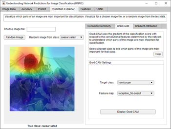
To explore applying these methods interactively using an app, see the Explore Deep Network Explainability Using an App GitHub® repository.
Interpretability Methods for Nonimage Data
Many interpretability focus on interpreting image classification or regression networks.
Interpreting nonimage data is often more challenging due to the nonvisual nature of the data.
You can use Grad-CAM to visualize the classification decisions of a 1-D convolutional network
trained on time series data. For more information, see Interpret Deep Learning Time-Series Classifications Using Grad-CAM. To explore the activations
of an LSTM network, use the activations and
tsne (Statistics and Machine Learning Toolbox) functions. For an example showing how to explore the predictions of an LSTM
network, see Visualize Activations of LSTM Network. To explore the behavior of a
network trained on tabular features, use the lime (Statistics and Machine Learning Toolbox) and shapley (Statistics and Machine Learning Toolbox) functions.
For an example showing how to interpret a feature input network, see Interpret Deep Network Predictions on Numeric Feature Data Using LIME. For more information about
interpreting machine learning models, see Interpret Machine Learning Models (Statistics and Machine Learning Toolbox).
References
[1] Zhou, Bolei, Aditya Khosla, Agata Lapedriza, Aude Oliva, and Antonio Torralba. "Learning Deep Features for Discriminative Localization." In 2016 Proceedings of the IEEE Conference on Computer Vision and Pattern Recognition : 2921–2929. Las Vegas: IEEE, 2016.
[2] Selvaraju, Ramprasaath R., Michael Cogswell, Abhishek Das, Ramakrishna Vedantam, Devi Parikh, and Dhruv Batra. “Grad-CAM: Visual Explanations from Deep Networks via Gradient-Based Localization.” In 2017 Proceedings of the IEEE Conference on Computer Vision: 618–626. Venice, Italy: IEEE, 2017. https://doi.org/10.1109/ICCV.2017.74.
[3] Ribeiro, Marco Tulio, Sameer Singh, and Carlos Guestrin. “‘Why Should I Trust You?’: Explaining the Predictions of Any Classifier.” In Proceedings of the 22nd ACM SIGKDD International Conference on Knowledge Discovery and Data Mining (2016): 1135–1144. New York, NY: Association for Computing Machinery, 2016. https://doi.org/10.1145/2939672.2939778.
[4] Simonyan, Karen, Andrea Vedaldi, and Andrew Zisserman. “Deep Inside Convolutional Networks: Visualising Image Classification Models and Saliency Maps.” Preprint, submitted April 19, 2014. https://arxiv.org/abs/1312.6034.
[5] Tomsett, Richard, Dan Harborne, Supriyo Chakraborty, Prudhvi Gurram, and Alun Preece. “Sanity Checks for Saliency Metrics.” Proceedings of the AAAI Conference on Artificial Intelligence, 34, no. 04, (April 2020): 6021–29, https://doi.org/10.1609/aaai.v34i04.6064.
[6] TensorFlow. "DeepDreaming with TensorFlow." https://github.com/tensorflow/docs/blob/master/site/en/tutorials/generative/deepdream.ipynb.
[7] van der Maaten, Laurens, and Geoffrey Hinton. "Visualizing Data Using t-SNE." Journal of Machine Learning Research, 9 (2008): 2579–2605.
See Also
dlnetwork | predict | forward | gradCAM | imageLIME | occlusionSensitivity | deepDreamImage | tsne (Statistics and Machine Learning Toolbox)
Topics
- Explore Network Predictions Using Deep Learning Visualization Techniques
- Grad-CAM Reveals the Why Behind Deep Learning Decisions
- Understand Network Predictions Using LIME
- Understand Network Predictions Using Occlusion
- View Network Behavior Using tsne
- Interpret Machine Learning Models (Statistics and Machine Learning Toolbox)