Rolling Element Bearing Fault Diagnosis Using Deep Learning
This example shows how to perform fault diagnosis of a rolling element bearing using a deep learning approach. The example demonstrates how to classify bearing faults by converting 1-D bearing vibration signals to 2-D images of scalograms and applying transfer learning using a pretrained network. Transfer learning significantly reduces the time spent on feature extraction and feature selection in conventional bearing diagnostic approaches, and provides good accuracy for the small MFPT data set used in this example.
To run this example, go to https://github.com/mathworks/RollingElementBearingFaultDiagnosis-Data, download the entire repository as a ZIP file, and save it in the same directory as the live script.
Rolling Element Bearing Faults
Localized faults in a rolling element bearing can occur in the outer race, the inner race, the cage, or a rolling element. High frequency resonances between the bearing and the response transducer are excited when the rolling elements strike a local fault on the outer or inner race, or a fault on a rolling element strikes the outer or inner race [1]. The following figure shows a rolling element striking a local fault at the inner race. A common problem is detecting and identifying these faults.

Machinery Failure Prevention Technology (MFPT) Challenge Data
MFPT Challenge data [2] contains 23 data sets collected from machines under various fault conditions. The first 20 data sets are collected from a bearing test rig, with three under good conditions, three with outer race faults under constant load, seven with outer race faults under various loads, and seven with inner race faults under various loads. The remaining three data sets are from real-world machines: an oil pump bearing, an intermediate speed bearing, and a planet bearing. The fault locations are unknown. In this example, you use only the data collected from the test rig with known conditions.
Each data set contains an acceleration signal gs, sampling rate sr, shaft speed rate, load weight load, and four critical frequencies representing different fault locations: ball pass frequency outer race (BPFO), ball pass frequency inner race (BPFI), fundamental train frequency (FTF), and ball spin frequency (BSF). The formulas for BPFO and BPFI are as follows [1].
BPFO:
BPFI:
As shown in the figure, is the ball diameter and is the pitch diameter. The variable is the shaft speed, is the number of rolling elements, and is the bearing contact angle [1].
Scalogram of Bearing Data
To benefit from pretrained CNN deep networks, use the plotBearingSignalAndScalogram helper function to convert 1-D vibration signals in the MFPT dataset to 2-D scalograms. A scalogram is a time-frequency domain representation of the original time-domain signal [3]. The two dimensions in a scalogram image represent time and frequency. To visualize the relationship between a scalogram and its original vibration signal, plot the vibration signal with an inner race fault against its scalogram.
% Import data with inner race fault
data_inner = load(fullfile(matlabroot, 'toolbox', 'predmaint', ...
    'predmaintdemos', 'bearingFaultDiagnosis', ...
    'train_data', 'InnerRaceFault_vload_1.mat'));
% Plot bearing signal and scalogram
plotBearingSignalAndScalogram(data_inner)

During the 0.1 seconds shown in the plot, the vibration signal contains 12 impulses because the tested bearing's BPFI is 118.875 Hz. Accordingly, the scalogram shows 12 distinct peaks that align with the impulses in the vibration signal. Next, visualize scalograms for the outer race fault.
% Import data with outer race fault
data_outer = load(fullfile(matlabroot, 'toolbox', 'predmaint', ...
    'predmaintdemos', 'bearingFaultDiagnosis', ...
    'test_data', 'OuterRaceFault_3.mat'));
% Plot original signal and its scalogram
plotBearingSignalAndScalogram(data_outer)

The scalogram of the outer race fault shows 8 distinct peaks during the first 0.1 seconds, which is consistent with the ballpass frequencies. Because the impulses in the time-domain signal is not as dominant as in the inner race fault case, the distinct peaks in the scalogram show less contrast with the background. The scalogram of the normal condition does not show dominant distinct peaks.
% Import normal bearing data
data_normal = load(fullfile(matlabroot, 'toolbox', 'predmaint', ...
    'predmaintdemos', 'bearingFaultDiagnosis', ...
    'train_data', 'baseline_1.mat'));
% Plot original signal and its scalogram
plotBearingSignalAndScalogram(data_normal)

The number of distinct peaks is a good feature to differentiate between inner race faults, outer race faults, and normal conditions. Therefore, a scalogram can be a good candidate for classifying bearing faults. In this example, all bearing signal measurements come from tests using the same shaft speed. To apply this example to bearing signals under different shaft speeds, the data needs to be normalized by shaft speed. Otherwise, the number of "pillars" in the scalogram will be wrong.
Prepare Training Data
Unzip the downloaded file.
if exist('RollingElementBearingFaultDiagnosis-Data-master.zip', 'file')
    unzip('RollingElementBearingFaultDiagnosis-Data-master.zip')
end
The downloaded dataset contains a training dataset with 14 MAT-files (2 normal, 5 inner race fault, 7 outer race fault) and a testing dataset with 6 MAT-files (1 normal, 2 inner race fault, 3 outer race fault).
By assigning function handles to ReadFcn, the file ensemble datastore can navigate into the files to retrieve data in the desired format. For example, the MFPT data has a structure bearing that stores the vibration signal gs, sampling rate sr, and so on. Instead of returning the bearing structure itself, the readMFPTBearing function is written so that the file ensemble datastore returns the vibration signal gs inside of the bearing data structure.
fileLocation = fullfile('.', 'RollingElementBearingFaultDiagnosis-Data-master', 'train_data');
fileExtension = '.mat';
ensembleTrain = fileEnsembleDatastore(fileLocation, fileExtension);
ensembleTrain.ReadFcn = @readMFPTBearing;
ensembleTrain.DataVariables = ["gs", "sr", "rate", "load", "BPFO", "BPFI", "FTF", "BSF"];
ensembleTrain.ConditionVariables = ["Label", "FileName"];
ensembleTrain.SelectedVariables = ["gs", "sr", "rate", "load", "BPFO", "BPFI", "FTF", "BSF", "Label", "FileName"]
ensembleTrain =
  fileEnsembleDatastore with properties:

                 ReadFcn: @readMFPTBearing
        WriteToMemberFcn: []
           DataVariables: [8×1 string]
    IndependentVariables: [0×0 string]
      ConditionVariables: [2×1 string]
       SelectedVariables: [10×1 string]
                ReadSize: 1
              NumMembers: 14
          LastMemberRead: [0×0 string]
                   Files: [14×1 string]
Now, convert the 1-D vibration signals to scalograms and save the images for training. The size of each scalogram is 227-by-227-by-3, which is the same input size required by SqueezeNet. To improve accuracy, the helper function convertSignalToScalogram envelops the raw signal and divides it into multiple segments. After running the following commands, a folder named "train_image" appears in the current folder. All scalogram images of the bearing signals in the "RollingElementBearingFaultDiagnosis-Data-master/train_data" folder are saved in the "train_image" folder.
reset(ensembleTrain)
while hasdata(ensembleTrain)
  folderName = 'train_image';
  convertSignalToScalogram(ensembleTrain,folderName);
end
Create an image datastore and split the training data into training and validation data sets, using 80% of the images from the "train_image" folder for training and 20% for validation.
% Create image datastore to store all training images
path = fullfile('.', folderName);
imds = imageDatastore(path, ...
  'IncludeSubfolders',true,'LabelSource','foldernames');
% Use 20% training data as validation set
[imdsTrain,imdsValidation] = splitEachLabel(imds,0.8,'randomize');
Train Network with Transfer Learning
Next, fine-tune the pretrained SqueezeNet convolutional neural network to perform classification on the scalograms. SqueezeNet has been trained on over a million images and has learned rich feature representations. Transfer learning is commonly used in deep learning applications. You can take a pretrained network and use it as a starting point for a new task. Fine-tuning a network with transfer learning is usually much faster and easier than training a network with randomly initialized weights from scratch. You can quickly transfer learned features using a smaller number of training images. Load and view the SqueezeNet network:
net = imagePretrainedNetwork("squeezenet")net =
dlnetwork with properties:
Layers: [68×1 nnet.cnn.layer.Layer]
Connections: [75×2 table]
Learnables: [52×3 table]
State: [0×3 table]
InputNames: {'data'}
OutputNames: {'prob_flatten'}
Initialized: 1
View summary with summary.
analyzeNetwork(net)
SqueezeNet uses the convolutional layer 'conv10' to extract image features and classify the input image. This layer contains information to combine the features that the network extracts into class probabilities, a loss value, and predicted labels. To retrain SqueezeNet for classifying new images, the convolutional layers 'conv10' need to be replaced with a new layer adapted to the bearing images.
In most networks, the last layer with learnable weights is a fully connected layer. In some networks, such as SqueezeNet, the last learnable layer is a 1-by-1 convolutional layer instead. In this case, replace the convolutional layer with a new convolutional layer with a number of filters equal to the number of classes.
numClasses = numel(categories(imdsTrain.Labels));

newConvLayer = convolution2dLayer([1, 1],numClasses,'WeightLearnRateFactor',10,'BiasLearnRateFactor',10,"Name",'new_conv');
net = replaceLayer(net,'conv10',newConvLayer);
Specify the training options. To slow down learning in the transferred layers, set the initial learning rate to a small value. When you create the convolutional layer, you include larger learning rate factors to speed up learning in the new final layers. This combination of learning rate settings results in fast learning only in the new layers and slower learning in the other layers. When performing transfer learning, you do not need to train for as many epochs. An epoch is a full training cycle on the entire training data set. The software validates the network every ValidationFrequency iterations during training.
options = trainingOptions('sgdm', ...
  'InitialLearnRate',0.0001, ...
  'MaxEpochs',4, ...
  'Shuffle','every-epoch', ...
  'ValidationData',imdsValidation, ...
  'ValidationFrequency',30, ...
  'Verbose',false, ...
  'MiniBatchSize',20, ...
  'Plots','training-progress');
Train the new network and set the loss function to 'crossentropy' (for classification problems). By default, trainnet uses a GPU if you have Parallel Computing Toolbox™ and a supported GPU device. For information on supported devices, see GPU Computing Requirements (Parallel Computing Toolbox). Otherwise, trainnet uses a CPU. You can also specify the execution environment by using the 'ExecutionEnvironment' name-value argument of trainingOptions.
net = trainnet(imdsTrain,net,"crossentropy",options);
Validate Using Test Data Sets
Use bearing signals in the "RollingElementBearingFaultDiagnosis-Data-master/test_data" folder to validate the accuracy of the trained network. The test data needs to be processed in the same way as the training data.
Create a file ensemble datastore to store the bearing vibration signals in the test folder.
fileLocation = fullfile('.', 'RollingElementBearingFaultDiagnosis-Data-master', 'test_data');
fileExtension = '.mat';
ensembleTest = fileEnsembleDatastore(fileLocation, fileExtension);
ensembleTest.ReadFcn = @readMFPTBearing;
ensembleTest.DataVariables = ["gs", "sr", "rate", "load", "BPFO", "BPFI", "FTF", "BSF"];
ensembleTest.ConditionVariables = ["Label", "FileName"];
ensembleTest.SelectedVariables = ["gs", "sr", "rate", "load", "BPFO", "BPFI", "FTF", "BSF", "Label", "FileName"];
Convert 1-D signals to 2-D scalograms.
reset(ensembleTest)
while hasdata(ensembleTest)
  folderName = 'test_image';
  convertSignalToScalogram(ensembleTest,folderName);
end
Create an image datastore to store the test images.
path = fullfile('.','test_image');
imdsTest = imageDatastore(path, ...
  'IncludeSubfolders',true,'LabelSource','foldernames');
Classify the test image datastore with the trained network.
scores = minibatchpredict(net,imdsTest,'MiniBatchSize',20);
YPred = scores2label(scores,unique(imdsTrain.Labels));
Compute the accuracy of the prediction.
YTest = imdsTest.Labels;
accuracy = sum(YPred == YTest)/numel(YTest)
accuracy = 0.9742
Plot a confusion matrix.
figure
confusionchart(YTest,YPred)
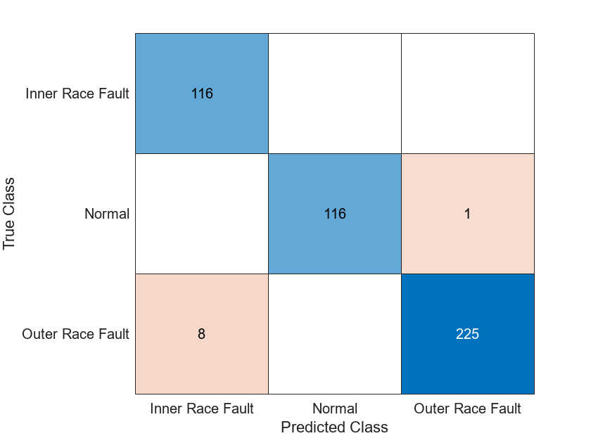
When you train the network multiple times, you might see some variation in accuracy between trainings, but the average accuracy should be around 98%. Even though the training set is quite small, this example benefits from transfer learning and achieves good accuracy.
Conclusion
This example demonstrates that deep learning can be an effective tool to identify different types of faults in rolling element bearing, even when the data size is relatively small. A deep learning approach reduces the time that conventional approach requires for feature engineering. For comparison, see the example Rolling Element Bearing Fault Diagnosis (Predictive Maintenance Toolbox).
References
[1] Randall, Robert B., and Jérôme Antoni. “Rolling Element Bearing Diagnostics—A Tutorial.” Mechanical Systems and Signal Processing 25, no. 2 (February 2011): 485–520. https://doi.org/10.1016/j.ymssp.2010.07.017.
[2] Bechhoefer, Eric. "Condition Based Maintenance Fault Database for Testing Diagnostics and Prognostic Algorithms." 2013. https://www.mfpt.org/fault-data-sets/.
[3] Verstraete, David, Andrés Ferrada, Enrique López Droguett, Viviana Meruane, and Mohammad Modarres. “Deep Learning Enabled Fault Diagnosis Using Time-Frequency Image Analysis of Rolling Element Bearings.” Shock and Vibration 2017 (2017): 1–17. https://doi.org/10.1155/2017/5067651.
Helper Functions
function plotBearingSignalAndScalogram(data)
% Convert 1-D bearing signals to scalograms through wavelet transform
fs = data.bearing.sr;
t_total = 0.1; % seconds
n = round(t_total*fs);
bearing = data.bearing.gs(1:n);
[cfs,frq] = cwt(bearing,'amor', fs);

% Plot the original signal and its scalogram
figure
subplot(2,1,1)
plot(0:1/fs:(n-1)/fs,bearing)
xlim([0,0.1])
title('Vibration Signal')
xlabel('Time (s)')
ylabel('Amplitude')
subplot(2,1,2)
surface(0:1/fs:(n-1)/fs,frq,abs(cfs))
shading flat
xlim([0,0.1])
ylim([0,max(frq)])
title('Scalogram')
xlabel('Time (s)')
ylabel('Frequency (Hz)')
end

function convertSignalToScalogram(ensemble,folderName)
% Convert 1-D signals to scalograms and save scalograms as images
data = read(ensemble);
fs = data.sr;
x = data.gs{:};
label = char(data.Label);
fname = char(data.FileName);
ratio = 5000/97656;
interval = ratio*fs;
N = floor(numel(x)/interval);

% Create folder to save images
path = fullfile('.',folderName,label);
if ~exist(path,'dir')
  mkdir(path);
end

for idx = 1:N
  sig = envelope(x(interval*(idx-1)+1:interval*idx));
  cfs = cwt(sig,'amor', seconds(1/fs));
  cfs = abs(cfs);
  img = ind2rgb(round(rescale(flip(cfs),0,255)),jet(320));
  outfname = fullfile('.',path,[fname '-' num2str(idx) '.jpg']);
  imwrite(imresize(img,[227,227]),outfname);
end
end
See Also
trainnet | trainingOptions | dlnetwork | imagePretrainedNetwork | analyzeNetwork | convolution2dLayer | replaceLayer | minibatchpredict | scores2label | confusionchart
Topics
- Rolling Element Bearing Fault Diagnosis (Predictive Maintenance Toolbox)