Automated Parking Valet
This example shows how to construct an automated parking valet system. In this example, you learn about tools and techniques in support of path planning, trajectory generation, and vehicle control. While this example focuses on a MATLAB®-oriented workflow, these tools are also available in Simulink®. For a Simulink version of this example, see Automated Parking Valet in Simulink.
Overview
Automatically parking a car that is left in front of a parking lot is a challenging problem. The vehicle's automated systems are expected to take over control and steer the vehicle to an available parking spot. Such a function makes use of multiple on-board sensors. For example:
Front and side cameras for detecting lane markings, road signs (stop signs, exit markings, etc.), other vehicles, and pedestrians
Lidar and ultrasound sensors for detecting obstacles and calculating accurate distance measurements
Ultrasound sensors for obstacle detection
IMU and wheel encoders for dead reckoning
On-board sensors are used to perceive the environment around the vehicle. The perceived environment includes an understanding of road markings to interpret road rules and infer drivable regions, recognition of obstacles, and detection of available parking spots.
As the vehicle sensors perceive the world, the vehicle must plan a path through the environment towards a free parking spot and execute a sequence of control actions needed to drive to it. While doing so, it must respond to dynamic changes in the environment, such as pedestrians crossing its path, and readjust its plan.
This example implements a subset of features required to implement such a system. It focuses on planning a feasible path through the environment, and executing the actions needed to traverse the path. Map creation and dynamic obstacle avoidance are excluded from this example.
% Set random number generator seed for reproducibility.
randSeed = rng(0);
cl = onCleanup(@()rng(randSeed));
Environment Model
The environment model represents a map of the environment. For a parking valet system, this map includes available and occupied parking spots, road markings, and obstacles such as pedestrians or other vehicles. Occupancy maps are a common representation for this form of environment model. Such a map is typically built using Simultaneous Localization and Mapping (SLAM) by integrating observations from lidar and camera sensors. This example concentrates on a simpler scenario, where a map is already provided, for example, by a vehicle-to-infrastructure (V2X) system or a camera overlooking the entire parking space. It uses a static map of a parking lot and assumes that the self-localization of the vehicle is accurate.
The parking lot example used in this example is composed of three occupancy grid layers.
Stationary obstacles: This layer contains stationary obstacles like walls, barriers, and bounds of the parking lot.
Road markings: This layer contains occupancy information pertaining to road markings, including road markings for parking spaces.
Parked cars: This layer contains information about which parking spots are already occupied.
Each map layer contains different kinds of obstacles that represent different levels of danger for a car navigating through it. With this structure, each layer can be handled, updated, and maintained independently.
Load and display the three map layers. In each layer, dark cells represent occupied cells, and light cells represent free cells.
mapLayers = loadParkingLotMapLayers;
plotMapLayers(mapLayers)

% For simplicity, combine the three layers into a single costmap.
costmap = combineMapLayers(mapLayers);

figure
plot(costmap, Inflation="off");
legend off


The combined costmap is a vehicleCostmapOccupiedThreshold property, and free if its cost is lower than the FreeThreshold property.
The costmap covers the entire 75m-by-50m parking lot area, divided into 0.5m-by-0.5m square cells.
costmap.MapExtent % [x, width, y, height] in meters

costmap.CellSize  % cell size in meters
ans =

     0    75     0    50


ans =

    0.5000
Create a vehicleDimensions
vehicleDims      = vehicleDimensions;
maxSteeringAngle = 35; % in degrees
Update the VehicleDimensions property of the costmap collision checker with the dimensions of the vehicle to park. This setting adjusts the extent of the inflation in the map around obstacles to correspond to the size of the vehicle being parked, ensuring that collision-free paths can be found through the parking lot.
costmap.CollisionChecker.VehicleDimensions = vehicleDims;
Define the starting pose of the vehicle. The pose is obtained through localization, which is left out of this example for simplicity. The vehicle pose is specified as ![$[x,y,\theta]$](../../examples/driving/win64/ParkingValetExample_eq02846632807081234914.png) , in world coordinates.
, in world coordinates.  represents the position of the center of the vehicle's rear axle in world coordinate system.
  represents the orientation of the vehicle with respect to world X axis. For more details, see Coordinate Systems in Automated Driving Toolbox.
currentPose = [4 12 0]; % [x, y, theta]
Behavioral Layer
Planning involves organizing all pertinent information into hierarchical layers. Each successive layer is responsible for a more fine-grained task. The behavioral layer [1] sits at the top of this stack. It is responsible for activating and managing the different parts of the mission by supplying a sequence of navigation tasks. The behavioral layer assembles information from all relevant parts of the system, including:
Localization: The behavioral layer inspects the localization module for an estimate of the current location of the vehicle.
Environment model: Perception and sensor fusion systems report a map of the environment around the vehicle.
Determining a parking spot: The behavioral layer analyzes the map to determine the closest available parking spot.
Finding a global route: A routing module calculates a global route through the road network obtained either from a mapping service or from a V2X infrastructure. Decomposing the global route as a series of road links allows the trajectory for each link to be planned differently. For example, the final parking maneuver requires a different speed profile than the approach to the parking spot. In a more general setting, this becomes crucial for navigating through streets that involve different speed limits, numbers of lanes, and road signs.
Rather than rely on vehicle sensors to build a map of the environment, this example uses a map that comes from a smart parking lot via V2X communication. For simplicity, assume that the map is in the form of an occupancy grid, with road links and locations of available parking spots provided by V2X.
The HelperBehavioralPlanner.m class mimics an interface of a behavioral planning layer. The HelperBehavioralPlanner.m is created using the map and the global route plan. This example uses a static global route plan stored in a MATLAB table, but typically a routing algorithm provided by the local parking infrastructure, or a mapping service determines this plan. The global route plan is described as a sequence of lane segments to traverse to reach a parking spot.
Load the MAT-file containing a route plan that is stored in a table. The table has three variables: StartPose, EndPose, and Attributes. StartPose and EndPose specify the start and end poses of the segment, expressed as . Attributes specifies properties of the segment such as the speed limit.
data = load("routePlan.mat");
routePlan = data.routePlan %#ok<NOPTS>
routePlan =

  3×3 table

      StartPose           EndPose         Attributes
    ______________    ________________    __________

     4    12     0    60     11      0    1×1 struct
    60    11     0    70     28     90    1×1 struct
    70    28    90    53     39    180    1×1 struct
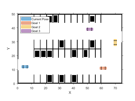
Plot a vehicle at the current pose, and along each goal in the route plan.
% Plot vehicle at current pose
hold on
helperPlotVehicle(currentPose, vehicleDims, DisplayName="Current Pose")
legend(Location="northwest")

for n = 1 : height(routePlan)
    % Extract the goal waypoint
    vehiclePose = routePlan{n, "EndPose"};

    % Plot the pose
    legendEntry = "Goal " + n;
    helperPlotVehicle(vehiclePose, vehicleDims, DisplayName=legendEntry);
end
hold off
Create the behavioral planner helper object. The requestManeuver method requests a stream of navigation tasks from the behavioral planner until the destination is reached.
behavioralPlanner = HelperBehavioralPlanner(routePlan, maxSteeringAngle);
The vehicle navigates each path segment using these steps:
Motion Planning: Plan a feasible path through the environment map using the optimal Hybrid A* algorithm
plannerHybridAStar(Navigation Toolbox)Local Path Optimization: Optimize the local path by maintaining a smooth curvature and a safe distance from obstacles using
controllerTEB(Navigation Toolbox)Vehicle Control: Given the smoothed reference path,
HelperPathAnalyzer.mcalculates the reference pose and velocity based on the current pose and velocity of the vehicle. Provided with the reference values,lateralControllerStanleyHelperLongitudinalController.mcomputes the acceleration and deceleration commands to maintain the desired vehicle velocity.Goal Checking: Check if the vehicle has reached the final pose of the segment using
helperGoalChecker.m.
The rest of this example describes these steps in detail, before assembling them into a complete solution.
Global Motion Planning with A* Planner
Given a global route, motion planning can be used to plan a path through the environment to reach each intermediate waypoint, until the vehicle reaches the final destination. The planned path for each link must be feasible and collision-free. A feasible path is one that can be realized by the vehicle given the motion and dynamic constraints imposed on it. A parking valet system involves low velocities and low accelerations. This allows us to safely ignore dynamic constraints arising from inertial effects.
Create a stateSpaceSE2 (Navigation Toolbox)-pi to pi radians.
ss = stateSpaceSE2;
ss.StateBounds = [costmap.MapExtent(1, 1:2); costmap.MapExtent(1, 3:4); -pi, pi];
Create a state validator validatorVehicleCostmap (Navigation Toolbox)
validator = validatorVehicleCostmap(ss, Map=costmap);
Create a plannerHybridAStar (Navigation Toolbox)
minTurningRadius = 10; % in meters
motionPlanner = plannerHybridAStar(validator, MinTurningRadius=minTurningRadius, ...
    MotionPrimitiveLength=4); % length in meters
Plan a path from the current pose to the first goal by using the plan function. The returned navPath (Navigation Toolbox)refPath, is a feasible and collision-free reference path. Note that plannerHybridAStar represents the vehicle orientation using radians rather than degrees.
goalPose = routePlan{1, "EndPose"};
currentPoseRad = [currentPose(1:2) deg2rad(currentPose(3))];
goalPoseRad = [goalPose(1:2) deg2rad(goalPose(3))];
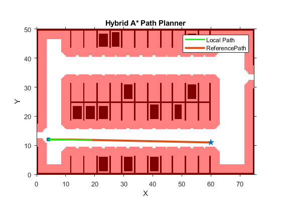
refPath = plan(motionPlanner, currentPoseRad, goalPoseRad);
plannerAxes = show(motionPlanner, Tree="off", HeadingLength=0); % Visualize the planned path.

In addition to the planned reference path, notice the red areas on the plot. These areas represent areas of the costmap where the origin of the vehicle (center of the rear axle) must not cross to avoid hitting any obstacles. plannerHybridAStar finds paths that avoid obstacles by checking to ensure that generated vehicle poses do not lie on these areas.
Local Trajectory Generation with Time Elastic Band Algorithm
The reference path generated by the path planner is composed of [x, y, theta] waypoints for the vehicle to follow. The reference path is achievable following the vehicle's nonholonomic constraints but does not consider passenger comfort and may result in abrupt changes to the steering angle. To avoid such unnatural motion and to ensure passenger comfort, use an optimization-based approach to find the optimum local trajectory based on the environment, vehicle constraints, and passenger comfort requirements.
Use the controllerTEB (Navigation Toolbox)controllerTEB planner uses the Time Elastic Band (TEB) algorithm to generate an optimized, smooth trajectory and maintain a safe distance from obstacles known or unknown to the global planner. The object also computes velocity commands and an optimal trajectory using the current pose of the vehicle and its current linear and angular velocities.
weights = struct(Time=10, Smoothness=100, Obstacle=50);
vehicleInfo = struct("Dimension", [vehicleDims.Length, vehicleDims.Width], "Shape", "Rectangle");

localPlanner = controllerTEB(zeros(3,3),...
    MaxVelocity=[5 0.5],... % in m/s and rad/s
    MaxAcceleration=[2 0.5],... % in m/s/s and rad/s/s
    LookAheadTime=3,... % in seconds
    MinTurningRadius=minTurningRadius, NumIteration=2,...
    CostWeights=weights, RobotInformation=vehicleInfo);
Plan a local trajectory starting at the current pose and closely following the reference path using the controllerTEB object.
% The local planner does not require knowledge of the full parking lot map
% since it is only planning a short local trajectory. Providing the local
% planner with a smaller map increases planner performance.
maxLocalPlanDistance = 15; % in meters
localPlanner.Map = getLocalMap(costmap, currentPose, maxLocalPlanDistance);
localPlanner.ReferencePath = refPath;

% Along with an optimized trajectory, |localPath|, the local planner provides
% a reference velocity for each point on the path, |refVel|.
[refVel, ~, localPath, ~] = localPlanner(currentPoseRad, [0 0]);

% Show the local trajectory alongside the reference path.
hold(plannerAxes,"on");
plot(plannerAxes, localPath(:,1), localPath(:,2), "g", LineWidth=2, DisplayName="Local Path");
legend(plannerAxes, "show", findobj(plannerAxes, Type="Line"), {"Local Path","ReferencePath"});
Vehicle Control and Simulation
The reference speeds, together with the smoothed path, comprise a feasible trajectory that the vehicle can follow. A feedback controller is used to follow this trajectory. The controller corrects errors in tracking the trajectory that arise from tire slippage and other sources of noise, such as inaccuracies in localization. In particular, the controller consists of two components:
Lateral control: Adjust the steering angle such that the vehicle follows the reference path.
Longitudinal control: While following the reference path, maintain the desired speed by controlling the throttle and the brake.
Since this scenario involves slow speeds, you can simplify the controller to consider only a kinematic model. In this example, lateral control is realized by the lateralControllerStanleyHelperLongitudinalController.m, that computes acceleration and deceleration commands based on the Proportional-Integral law.
The feedback controller requires a simulator that can execute the desired controller commands using a suitable vehicle model. The HelperVehicleSimulator.m class simulates such a vehicle using the following kinematic bicycle model:


In the above equations,  represents the vehicle pose in world coordinates.
  ,
,  ,
,  , and
, and  represent the rear-wheel speed, rear-wheel acceleration, wheelbase, and steering angle, respectively. The position and speed of the front wheel can be obtained by:


closeFigures; % Close all

% Create the vehicle simulator.
vehicleSim = HelperVehicleSimulator(costmap, vehicleDims);

hideFigure(vehicleSim); % Hide vehicle simulation figure

% Configure the simulator to show the trajectory.
vehicleSim.showTrajectory(true);
vehicleSim.showLegend(true);

% Set the vehicle pose and velocity.
vehicleSim.setVehiclePose(currentPose);
currentVel = 0;
vehicleSim.setVehicleVelocity(currentVel);
Create a HelperPathAnalyzer.m object to compute reference pose, reference velocity and driving direction for the controller.
pathAnalyzer = HelperPathAnalyzer(Wheelbase=vehicleDims.Wheelbase);
Create a HelperLongitudinalController.m object to control the velocity of the vehicle and specify the sample time.
sampleTime = 0.05;
lonController = HelperLongitudinalController(SampleTime=sampleTime);
Use the HelperFixedRate.m object to ensure fixed-rate execution of the feedback controller. Use a control rate to be consistent with the longitudinal controller.
controlRate = HelperFixedRate(1/sampleTime); % in Hertz
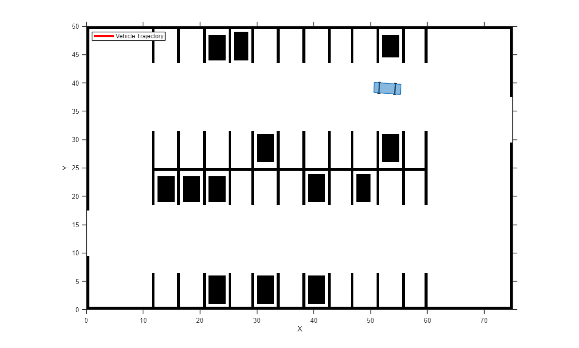
Execute a Complete Plan
Now combine all the previous steps in the planning process and run the simulation for the complete route plan. This process involves incorporating the behavioral planner.
% Set the vehicle pose back to the initial starting point.
currentPose = [4 12 0]; % [x, y, theta]
vehicleSim.setVehiclePose(currentPose);

% Reset velocity.
currentVel  = 0; % meters/second
vehicleSim.setVehicleVelocity(currentVel);

% Initialize variables to store vehicle path.
refPath = [];
localPath = [];

% Setup pathAnalyzer to trigger update of local path every 1 second.
localPlanningFrequency = 1; % 1/seconds
pathAnalyzer.PlanningPeriod = 1/localPlanningFrequency/sampleTime; % timesteps

isGoalReached = false;

% Initialize count incremented each time the local planner is updated
localPlanCount = 0; % Used for visualization only

showFigure(vehicleSim); % Show vehicle simulation figure.

while ~isGoalReached
    % Plan for the next path segment if near to the next path segment start
    % pose.
    if planNextSegment(behavioralPlanner, currentPose, 2*maxLocalPlanDistance)
        % Request next maneuver from behavioral layer.
        [nextGoal, plannerConfig, speedConfig] = requestManeuver(behavioralPlanner, ...
            currentPose, currentVel);

        % Plan a reference path using A* planner to the next goal pose.
        if isempty(refPath)
            nextStartRad = [currentPose(1:2) deg2rad(currentPose(3))];
        else
            nextStartRad = refPath(end,:);
        end
        nextGoalRad = [nextGoal(1:2) deg2rad(nextGoal(3))];
        newPath = plan(motionPlanner, nextStartRad, nextGoalRad, SearchMode="exhaustive");

        % Check if the path is valid. If the planner fails to compute a path,
        % or the path is not collision-free because of updates to the map, the
        % system needs to re-plan. This scenario uses a static map, so the path
        % will always be collision-free.
        isReplanNeeded = ~checkPathValidity(newPath.States, costmap);
        if isReplanNeeded
            warning("Unable to find a valid path. Attempting to re-plan.")

            % Request behavioral planner to re-plan
            replanNeeded(behavioralPlanner);
        else
            % Append to refPath
            refPath = [refPath; newPath.States];
            hasNewPath = true;

            vehicleSim.plotReferencePath(refPath); % Plot reference path
        end
    end

    % Update the local path at the frequency specified by
    % |localPlanningFrequency|
    if pathUpdateNeeded(pathAnalyzer)
        currentPose  = getVehiclePose(vehicleSim);
        currentPoseRad = [currentPose(1:2) deg2rad(currentPose(3))];
        currentVel   = getVehicleVelocity(vehicleSim);
        currentAngVel = getVehicleAngularVelocity(vehicleSim);

        % Do local planning
        localPlanner.Map = getLocalMap(costmap, currentPose, maxLocalPlanDistance);

        if hasNewPath
            localPlanner.ReferencePath = refPath;
            hasNewPath = false;
        end

        [localVel, ~, localPath, ~] = localPlanner(currentPoseRad, [currentVel currentAngVel]);

        vehicleSim.plotLocalPath(localPath); % Plot new local path

        % For visualization only
        if mod(localPlanCount, 20) == 0
            snapnow; % Capture state of the figures
        end
        localPlanCount = localPlanCount+1;

        % Configure path analyzer.
        pathAnalyzer.RefPoses     = [localPath(:,1:2) rad2deg(localPath(:,3))];
        pathAnalyzer.Directions   = sign(localVel(:,1));
        pathAnalyzer.VelocityProfile = localVel(:,1);
    end

    % Find the reference pose on the path and the corresponding
    % velocity.
    [refPose, refVel, direction] = pathAnalyzer(currentPose, currentVel);

    % Update driving direction for the simulator.
    updateDrivingDirection(vehicleSim, direction);

    % Compute steering command.
    steeringAngle = lateralControllerStanley(refPose, currentPose, currentVel, ...
        Direction=direction, Wheelbase=vehicleDims.Wheelbase, PositionGain=4);

    % Compute acceleration and deceleration commands.
    lonController.Direction = direction;
    [accelCmd, decelCmd] = lonController(refVel, currentVel);

    % Simulate the vehicle using the controller outputs.
    drive(vehicleSim, accelCmd, decelCmd, steeringAngle);

    % Get current pose and velocity of the vehicle.
    currentPose  = getVehiclePose(vehicleSim);
    currentVel   = getVehicleVelocity(vehicleSim);

    % Check if the vehicle reaches the goal.
    isGoalReached = helperGoalChecker(nextGoal, currentPose, currentVel, speedConfig.EndSpeed, direction);

    % Wait for fixed-rate execution.
    waitfor(controlRate);
end


Parking Maneuver
Now that the vehicle is near the parking spot, a specialized parking maneuver is used to park the vehicle in the parking spot. This maneuver requires passing through a narrow corridor flanked by the edges of the parking spot on both ends. Such a maneuver is typically accompanied with ultrasound sensors or laser scanners continuously checking for obstacles.
The vehicle navigates the parking maneuver using these steps:
Motion Planning: Plan a feasible path through the environment map using the optimal rapidly exploring random tree (RRT*) algorithm (
pathPlannerRRT).Path Smoothing: Smooth the reference path by fitting splines to it using
smoothPathSplineTrajectory Generation: Convert the smoothed path into a trajectory by generating a speed profile using
helperGenerateVelocityProfile.m.Vehicle Control: Given the smoothed reference path,
HelperPathAnalyzer.mcalculates the reference pose and velocity based on the current pose and velocity of the vehicle. Provided with the reference values,lateralControllerStanleyHelperLongitudinalController.mcomputes the acceleration and deceleration commands to maintain the desired vehicle velocity.Goal Checking: Check if the vehicle has reached the final pose of the segment using
helperGoalChecker.m.
hideFigure(vehicleSim); % Hide vehicle simulation figure
The vehicleCostmap uses inflation-based collision checking. First, visually inspect the current collision checker in use.
ccConfig = costmap.CollisionChecker;

figure
plot(ccConfig)
title("Current Collision Checker")

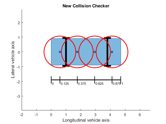
Collision checking is performed by inflating obstacles in the costmap by the inflation radius, and checking whether the center of the circle shown above lies on an inflated grid cell. The final parking maneuver requires a more precise, less conservative collision-checking mechanism. This is commonly solved by representing the shape of the vehicle using multiple (3-5) overlapping circles instead of a single circle.
Use a larger number of circles in the collision checker and visually inspect the collision checker. This allows planning through narrow passages.
ccConfig.NumCircles = 4;

figure
plot(ccConfig)
title("New Collision Checker")
Update the costmap to use this collision checker.
costmap.CollisionChecker = ccConfig;
Notice that the inflation radius has reduced, allowing the planner to find an unobstructed path to the parking spot.
figure
plot(costmap)
title("Costmap with updated collision checker")

Parking Maneuver Motion Planning with RRT Planner
Create a pathPlannerRRT
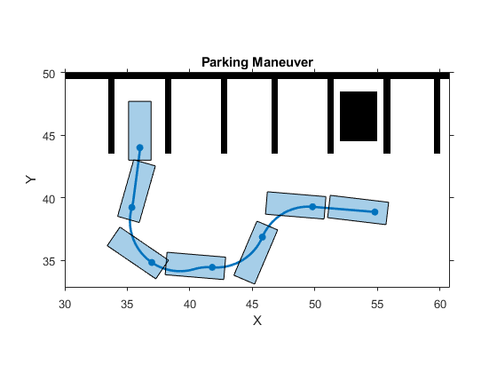
% Set up the pathPlannerRRT to use the updated costmap.
parkMotionPlanner = pathPlannerRRT(costmap, MinIterations=1000);

% Define desired pose for the parking spot, returned by the V2X system.
parkPose = [36 44 90];
preParkPose = currentPose;

% Compute the parking maneuver.
replan = true;
while replan
    % Compute the required parking maneuver.
    refPath = plan(parkMotionPlanner, preParkPose, parkPose);

    % Retrieve transition poses and directions from the planned path.
    [transitionPoses, directions] = interpolate(refPath);

    replan = isempty(refPath.PathSegments) || any(directions == -1) || refPath.Length > 30;
end

% Plot the resulting parking maneuver.
figure
plotParkingManeuver(costmap, refPath, preParkPose, parkPose)
Parking Maneuver Path Smoothing with Parametric Cubic Spline
The reference path generated by the path planner is composed either of Dubins or Reeds-Shepp segments. The curvature at the junctions of two such segments is not continuous and can result in abrupt changes to the steering angle. To avoid such unnatural motion and to ensure passenger comfort, the path needs to be continuously differentiable and therefore smooth [2]. One approach to smoothing a path involves fitting a parametric cubic spline. Spline fitting enables you to generate a smooth path that a controller can execute.
% Specify number of poses to return using a separation of approximately 1 m.
approxSeparation = 1; % meters

% Smooth the path.
numSmoothPoses   = round(refPath.Length / approxSeparation);
[refPoses, directions, cumLengths, curvatures] = smoothPathSpline(transitionPoses, directions, numSmoothPoses);

% Set up the velocity profile generator to stop at the end of the trajectory,
% with a speed limit of 5 mph.
refVelocities = helperGenerateVelocityProfile(directions, cumLengths, curvatures, currentVel, 0, 2.2352);
Simulate forward parking maneuver.
showFigure(vehicleSim); % Show vehicle simulation figure.
pathAnalyzer.RefPoses     = refPoses;
pathAnalyzer.Directions   = directions;
pathAnalyzer.VelocityProfile = refVelocities;

% Clear old path planning data from the plot
vehicleSim.clearReferencePath();
vehicleSim.clearLocalPath();

% Reset longitudinal controller.
reset(lonController);

isGoalReached = false;

while ~isGoalReached
    % Find the reference pose on the path and the corresponding velocity.
    [refPose, refVel, direction] = pathAnalyzer(currentPose, currentVel);

    % Update driving direction for the simulator.
    updateDrivingDirection(vehicleSim, direction);

    % Compute steering command.
    steeringAngle = lateralControllerStanley(refPose, currentPose, currentVel, ...
        Direction=direction, Wheelbase=vehicleDims.Wheelbase);

    % Compute acceleration and deceleration commands.
    lonController.Direction = direction;
    [accelCmd, decelCmd] = lonController(refVel, currentVel);

    % Simulate the vehicle using the controller outputs.
    drive(vehicleSim, accelCmd, decelCmd, steeringAngle);

    % Check if the vehicle reaches the goal.
    isGoalReached = helperGoalChecker(parkPose, currentPose, currentVel, 0, direction);

    % Wait for fixed-rate execution.
    waitfor(controlRate);

    % Get current pose and velocity of the vehicle.
    currentPose  = getVehiclePose(vehicleSim);
    currentVel   = getVehicleVelocity(vehicleSim);
end

closeFigures; % Close all

An alternative way to park the vehicle is to back into the parking spot. When the vehicle needs to back up into a spot, the motion planner needs to use the Reeds-Shepp connection method to search for a feasible path. The Reeds-Shepp connection allows for reverse motions during planning.
% Specify a parking pose corresponding to a back-in parking maneuver.
parkPose = [49 47.2 -90];

% Change the connection method to allow for reverse motions.
parkMotionPlanner.ConnectionMethod = "Reeds-Shepp";

To find a feasible path, the motion planner needs to be adjusted. Use a larger turning radius and connection distance to allow for a smooth back-in.
parkMotionPlanner.MinTurningRadius   = 12; % meters
parkMotionPlanner.ConnectionDistance = 15; % meters

% Reset vehicle pose and velocity.
currentVel = 0; % m/s
vehicleSim.setVehiclePose(preParkPose);
vehicleSim.setVehicleVelocity(currentVel);

% Compute the parking maneuver.
replan = true;
while replan
    refPath = plan(parkMotionPlanner, preParkPose, parkPose);

    % The path corresponding to the parking maneuver is small and requires
    % precise maneuvering. Instead of interpolating only at transition poses,
    % interpolate more finely along the length of the path.

    numSamples = 10;
    stepSize   = refPath.Length / numSamples;
    lengths    = 0 : stepSize : refPath.Length;

    [transitionPoses, directions] = interpolate(refPath, lengths);

    % Replan if the path contains more than one direction switching poses
    % or if the path is too long.
    replan = isempty(refPath.PathSegments) || sum(abs(diff(directions(1:end-1))))~=2 || refPath.Length > 25;
end

% Visualize the parking maneuver.
figure
plotParkingManeuver(costmap, refPath, preParkPose, parkPose)


% Smooth the path.
numSmoothPoses   = round(refPath.Length / approxSeparation);
minSeparation = 0.5;
[refPoses, directions, cumLengths, curvatures] = smoothPathSpline(transitionPoses, directions, numSmoothPoses, minSeparation);

% Set up the velocity profile generator to stop at the end of the trajectory,
% with a speed limit of 5 mph.
refVelocities = helperGenerateVelocityProfile(directions, cumLengths, curvatures, currentVel, 0, 2.2352);
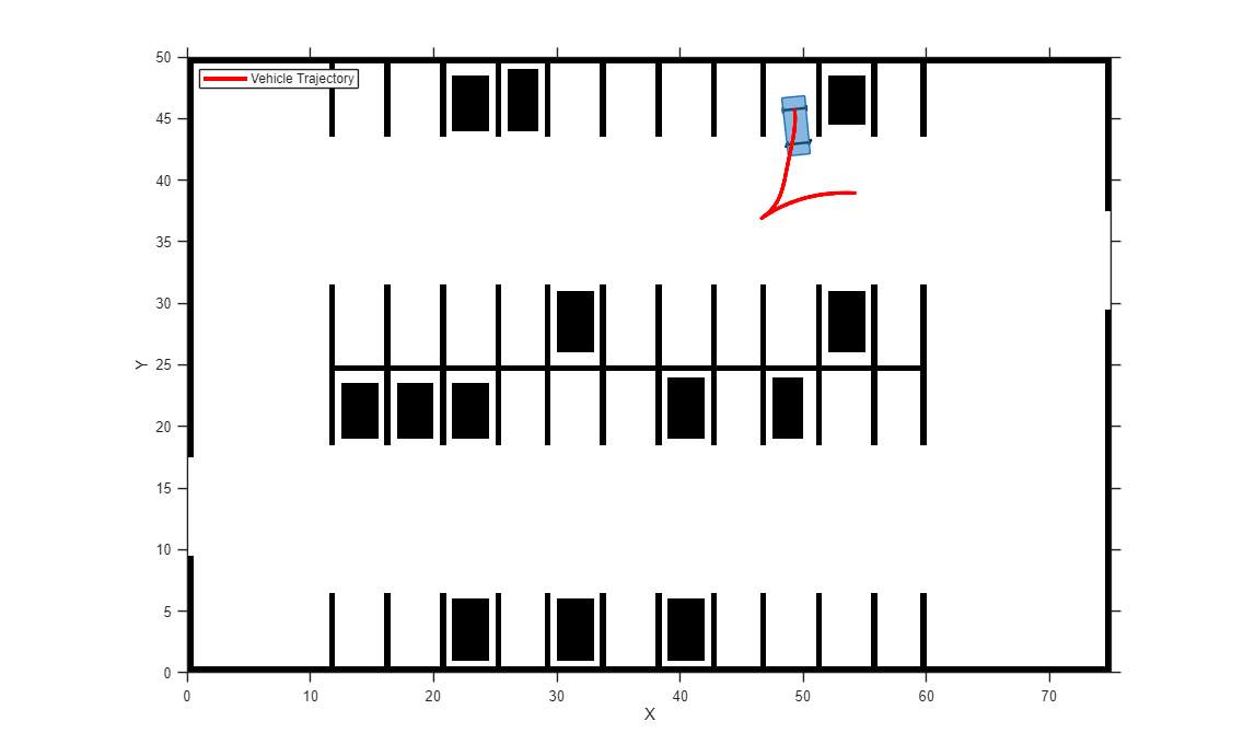
Simulate reverse parking maneuver.
pathAnalyzer.RefPoses     = refPoses;
pathAnalyzer.Directions   = directions;
pathAnalyzer.VelocityProfile = refVelocities;

reset(lonController); % Reset longitudinal controller.

isGoalReached = false;

while ~isGoalReached
    % Get current driving direction.
    currentDir = getDrivingDirection(vehicleSim);

    % Find the reference pose on the path and the corresponding velocity.
    [refPose, refVel, direction] = pathAnalyzer(currentPose, currentVel);

    % If the vehicle changes driving direction, reset vehicle velocity in
    % the simulator and reset longitudinal controller.
    if currentDir ~= direction
        currentVel = 0;
        setVehicleVelocity(vehicleSim, currentVel);
        reset(lonController);
    end

    % Update driving direction for the simulator. If the vehicle changes
    % driving direction, reset and return the current vehicle velocity as zero.
    currentVel = updateDrivingDirection(vehicleSim, direction, currentDir);

    % Compute steering command.
    steeringAngle = lateralControllerStanley(refPose, currentPose, currentVel, ...
        Direction=direction, Wheelbase=vehicleDims.Wheelbase);

    % Compute acceleration and deceleration commands.
    lonController.Direction = direction;
    [accelCmd, decelCmd] = lonController(refVel, currentVel);

    % Simulate the vehicle using the controller outputs.
    drive(vehicleSim, accelCmd, decelCmd, steeringAngle);

    % Check if the vehicle reaches the goal.
    isGoalReached = helperGoalChecker(parkPose, currentPose, currentVel, 0, direction);

    % Wait for fixed-rate execution.
    waitfor(controlRate);

    % Get current pose and velocity of the vehicle.
    currentPose  = getVehiclePose(vehicleSim);
    currentVel   = getVehicleVelocity(vehicleSim);
end

closeFigures;
snapnow; % Capture state of the simulation figure

delete(vehicleSim); % Delete the simulator.
Conclusion
This example showed how to:
Plan a feasible path in a semi-structured environment, such as a parking lot, using A* and RRT* path planning algorithms.
Find and optimized local trajectory or smooth the path using splines and generate a speed profile along the smoothed path.
Control the vehicle to follow the reference path at the desired speed.
Realize different parking behaviors by using different motion planner settings.
References
[1] Buehler, Martin, Karl Iagnemma, and Sanjiv Singh. The DARPA Urban Challenge: Autonomous Vehicles in City Traffic (1st ed.). Springer Publishing Company, Incorporated, 2009.
[2] Lepetic, Marko, Gregor Klancar, Igor Skrjanc, Drago Matko, Bostjan Potocnik, "Time Optimal Path Planning Considering Acceleration Limits." Robotics and Autonomous Systems. Volume 45, Issues 3-4, 2003, pp. 199-210.
Supporting Functions
loadParkingLotMapLayers Load environment map layers for parking lot
function mapLayers = loadParkingLotMapLayers()
% Load occupancy maps corresponding to 3 layers - obstacles, road
% markings, and used spots.

mapLayers.StationaryObstacles = imread("stationary.bmp");
mapLayers.RoadMarkings        = imread("road_markings.bmp");
mapLayers.ParkedCars          = imread("parked_cars.bmp");
end
plotMapLayers Plot struct containing map layers
function plotMapLayers(mapLayers)
%   Plot the multiple map layers on a figure window.

figure
cellOfMaps = cellfun(@imcomplement, struct2cell(mapLayers), UniformOutput=false);
montage(cellOfMaps, Size=[1 numel(cellOfMaps)], Border=[5 5], ThumbnailSize=[300 NaN])
title("Map Layers - Stationary Obstacles, Road markings, and Parked Cars")
end
combineMapLayers Combine map layers into a single costmap
function costmap = combineMapLayers(mapLayers)
% Combine map layers struct into a single vehicleCostmap.

combinedMap = mapLayers.StationaryObstacles + mapLayers.RoadMarkings + ...
    mapLayers.ParkedCars;
combinedMap = im2single(combinedMap);

costmap = vehicleCostmap(combinedMap, CellSize=0.5);
end
getLocalMap Extract area local to vehicle from costmap
function localMap = getLocalMap(costmap, pose, maxDistance)
% Extract area within maxDistance of pose from costmap

mapExtent = costmap.MapExtent;
cellSize = costmap.CellSize;
xMin = max(pose(1)-maxDistance, mapExtent(1));
xMax = min(pose(1)+maxDistance, mapExtent(2));
yMin = max(pose(2)-maxDistance, mapExtent(3));
yMax = min(pose(2)+maxDistance, mapExtent(4));

xMinCell = round(xMin/cellSize)+1;
xMaxCell = round(xMax/cellSize);
yMaxCell = costmap.MapSize(1) - round(yMin/cellSize);
yMinCell = costmap.MapSize(1) - round(yMax/cellSize)+1;

costs = getCosts(costmap);
localCosts = costs(yMinCell:yMaxCell, xMinCell:xMaxCell);
localMap = occupancyMap(localCosts, 1/cellSize);
localMap.GridLocationInWorld = [xMin yMin];
end
plotVelocityProfile Plot speed profile
function plotVelocityProfile(path, refVelocities, maxSpeed)
% Plot the generated velocity profile.

% Calculate cumulative path lengths
cumPathLength = pdist(path(:, 1:2));

% Plot reference velocity along length of the path.
plot(cumPathLength, refVelocities, LineWidth=2);

% Plot a line to display maximum speed.
hold on
line([0;cumPathLength(end)], [maxSpeed;maxSpeed], Color="r")
hold off

% Set axes limits.
buffer = 2;
xlim([0 cumPathLength(end)]);
ylim([0 maxSpeed + buffer])

% Add labels.
xlabel("Cumulative Path Length (m)");
ylabel("Velocity (m/s)");

% Add legend and title.
legend("Velocity Profile", "Max Speed")
title("Generated velocity profile")
end
closeFigures
function closeFigures()
% Close all the figures except the simulator visualization.

% Find all the figure objects.
figHandles = findobj(Type="figure");
for i = 1: length(figHandles)
    if ~strcmp(figHandles(i).Name, "Automated Valet Parking")
        close(figHandles(i));
    end
end
end
plotParkingManeuver Display the generated parking maneuver on a costmap.
function plotParkingManeuver(costmap, refPath, currentPose, parkPose)
% Plot the generated parking maneuver on a costmap.

% Plot the costmap, without inflated areas.
plot(costmap, Inflation="off")

% Plot reference parking maneuver on the costmap.
hold on
plot(refPath, DisplayName="Parking Maneuver")

title("Parking Maneuver")

% Zoom into parking maneuver by setting axes limits.
lo = min([currentPose(1:2); parkPose(1:2)]);
hi = max([currentPose(1:2); parkPose(1:2)]);

buffer = 6; % meters

xlim([lo(1)-buffer hi(1)+buffer])
ylim([lo(2)-buffer hi(2)+buffer])
end