Forecast State-Space Model Containing Regime Change in the Forecast Horizon
This example shows how to forecast a time-varying, state-space model, in which there is a regime change in the forecast horizon.
Suppose that you observed a multivariate process for 75 periods, and you want to forecast the process 25 periods into the future. Also, suppose that you can specify the process as a state-space model. For periods 1 through 50, the state-space model has one state: a stationary AR(2) model with a constant term. At period 51, the state-space model includes a random walk. The states are observed unbiasedly, but with additive measurement error. Symbolically, the model is
For periods 1 through 50, the random walk process is not in the model.
Specify the in-sample, coefficient matrices.
A1 = {[0.5 0.2 1; 1 0 0; 0 0 1]};                % A for periods 1 - 50
A2 = {[0.5 0.2 1; 1 0 0; 0 0 1; 0 0 0]};         % A for period 51
A3 = {[0.5 0.2 1 0; 1 0 0 0; 0 0 1 0; 0 0 0 1]}; % A for periods 51 - 75
A = [repmat(A1,50,1); A2; repmat(A3,24,1)];

B1 = {[0.1; 0; 0]};              % B for periods 1 - 50
B3 = {[0.1 0; 0 0; 0 0; 0 0.5]}; % B for periods 51 - 75
B = [repmat(B1,50,1); repmat(B3,25,1)];

C1 = {[1 0 0]};            % C for periods 1 - 50
C3 = {[1 0 0 0; 0 0 0 1]}; % C for periods 51 - 75
C = [repmat(C1,50,1); repmat(C3,25,1)];

D1 = {0.3};            % D for periods 1 - 50
D3 = {[0.3 0; 0 0.2]}; % D for periods 51 - 75
D = [repmat(D1,50,1); repmat(D3,25,1)];
Specify the state space model, and the initial state means and covariance matrix. It is best practice to specify the types of each state using the 'StateType' name-value pair argument. Only specify the initial state parameters for the three states that start the state-space model.
Mean0 = [1/(1-0.5-0.2); 1/(1-0.5-0.2); 1];
Cov0 = [0.02 0.01 0; 0.01 0.02 0; 0 0 0];
StateType = [0; 0; 1];
Mdl = ssm(A,B,C,D,'Mean0',Mean0,'Cov0',Cov0,'StateType',StateType)
Mdl =
State-space model type: ssm

State vector length: Time-varying
Observation vector length: Time-varying
State disturbance vector length: Time-varying
Observation innovation vector length: Time-varying
Sample size supported by model: 75

State variables: x1, x2,...
State disturbances: u1, u2,...
Observation series: y1, y2,...
Observation innovations: e1, e2,...

State equations of period 1, 2, 3,..., 50:
x1(t) = (0.50)x1(t-1) + (0.20)x2(t-1) + x3(t-1) + (0.10)u1(t)
x2(t) = x1(t-1)
x3(t) = x3(t-1)

State equations of period 51:
x1(t) = (0.50)x1(t-1) + (0.20)x2(t-1) + x3(t-1) + (0.10)u1(t)
x2(t) = x1(t-1)
x3(t) = x3(t-1)
x4(t) = (0.50)u2(t)

State equations of period 52, 53, 54,..., 75:
x1(t) = (0.50)x1(t-1) + (0.20)x2(t-1) + x3(t-1) + (0.10)u1(t)
x2(t) = x1(t-1)
x3(t) = x3(t-1)
x4(t) = x4(t-1) + (0.50)u2(t)


Observation equation of period 1, 2, 3,..., 50:
y1(t) = x1(t) + (0.30)e1(t)

Observation equations of period 51, 52, 53,..., 75:
y1(t) = x1(t) + (0.30)e1(t)
y2(t) = x4(t) + (0.20)e2(t)


Initial state distribution:

Initial state means
  x1    x2   x3
 3.33  3.33   1

Initial state covariance matrix
     x1    x2    x3
 x1  0.02  0.01   0
 x2  0.01  0.02   0
 x3   0     0     0

State types
     x1          x2         x3
 Stationary  Stationary  Constant
Mdl is a time-varying, ssm model without unknown parameters. The software sets initial state means and covariance values based on the type of state.
Simulate 75 observations from Mdl.
rng(1); % For reproducibility
Y = simulate(Mdl,75);
y is a 75-by-1 cell vector. Cells 1 through 50 contain scalars, and cells 51 through 75 contain 2-by-1 numeric vectors. Cell j corresponds to the observations of period j, specified by the observation model.
Plot the simulated responses.
y1 = cell2mat(Y(51:75));              % Observations for periods 1 - 50
d1 = cell2mat(Y(51:75));
y2 = [d1(((1:25)*2)-1) d1((1:25)*2)]; % Observations for periods 51 - 75

figure
plot(1:75,[y1;y2(:,1)],'-k',1:75,[nan(50,1);y2(:,2)],'-r','LineWidth',2')
title('In-sample Observations')
ylabel('Observations')
xlabel('Period')
legend({'AR(2)','Random walk'})
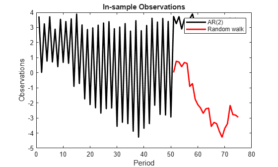
Suppose that the random walk process drops out of the state space in the 20th period of the forecast horizon.
Specify the coefficient matrices for the forecast period.
A4 = {[0.5 0.2 1 0; 1 0 0 0; 0 0 1 0; 0 0 0 1]};  % A for periods 76 - 95
A5 = {[0.5 0.2 1 0; 1 0 0 0; 0 0 1 0]};           % A for period 96
A6 = {[0.5 0.2 1; 1 0 0; 0 0 1]};                 % A for periods 97 - 100
fhA = [repmat(A4,20,1); A5; repmat(A6,4,1)];

B4 = {[0.1 0; 0 0; 0 0; 0 0.5]}; % B for periods 76 - 95
B6 = {[0.1; 0; 0]};              % B for periods 96 - 100
fhB = [repmat(B4,20,1); repmat(B6,5,1)];

C4 = {[1 0 0 0; 0 0 0 1]}; % C for periods 76 - 95
C6 = {[1 0 0]};            % C for periods 96 - 100
fhC = [repmat(C4,20,1); repmat(C6,5,1)];

D4 = {[0.3 0; 0 0.2]}; % D for periods 76 - 95
D6 = {0.3};            % D for periods 96 - 100
fhD = [repmat(D4,20,1); repmat(D6,5,1)];
Forecast observations over the forecast horizon.
FY = forecast(Mdl,25,Y,'A',fhA,'B',fhB,'C',fhC,'D',fhD);
FY is a 25-by-1 cell vector. Cells 1 through 20 contain 2-by-1 numeric vectors, and cells 51 through 75 contain scalars. Cell j corresponds to the observations of period j, specified by the forecast-horizon, observation model.
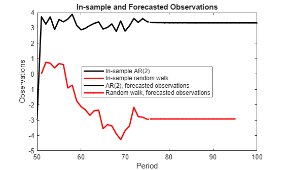
Plot the forecasts with the in-sample observations.
d2 = cell2mat(FY(1:20));
FY1 = [d2(((1:20)*2)-1) d2((1:20)*2)]; % Forecasts for periods 76 - 95
FY2 = cell2mat(FY(21:25));             % Forecasts for periods 96 - 100

figure
plot(1:75,[y1;y2(:,1)],'-k',1:75,[nan(50,1);y2(:,2)],'-r',...
    76:100,[FY1(:,1); FY2],'.-k',76:100,[FY1(:,2); nan(5,1)],'.-r',...
    75:76,[y2(end,1) FY1(1,1)],':k',75:76,[y2(end,2) FY1(1,2)],':r',...
    'LineWidth',2')
title('In-sample and Forecasted Observations')
ylabel('Observations')
xlabel('Period')
xlim([50,100])
legend({'In-sample AR(2)','In-sample random walk',...
    'AR(2), forecasted observations',...
    'Random walk, forecasted observations'},'Location','Best')%% Title
See Also
ssm | estimate | forecast | refine
Topics
- Implicitly Create Time-Varying State-Space Model
- Estimate Time-Varying State-Space Model
- Forecast State-Space Model Observations
- Forecast Time-Varying State-Space Model
- Forecast Observations of State-Space Model Containing Regression Component
- Forecast State-Space Model Using Monte-Carlo Methods
- Create Continuous State-Space Models for Economic Data Analysis
- What Is the Kalman Filter?