gctest
Granger causality and block exogeneity tests for vector autoregression (VAR) models
Description
The gctest object function can conduct leave-one-out,
exclude-all, and block-wise Granger causality tests for the
response variables of a fully specified vector autoregression (VAR)
model (represented by a varm model object).
To conduct a block-wise Granger causality test from specified sets of time series data
representing "cause" and "effect" multivariate response variables, or to address possibly
integrated series for the test, see the gctest
function.
h = gctest(Mdl)h from conducting leave-one-out Granger causality tests on all
response variables that compose the VAR(p) model
Mdl.
h = gctest(Mdl,Name,Value)'Type',"block-wise",'Cause',1:2,'Effect',3:5 specifies conducting a
block-wise test to assess whether the response variables
Mdl.SeriesNames(1:2) Granger-cause the response variables
Mdl.SeriesNames(3:5) conditioned on all other variables in the
model.
Examples
Conduct a leave-one-out Granger causality test to assess whether each variable in a 3-D VAR model Granger-causes another variable, given the third variable. The variables in the VAR model are the M1 money supply, consumer price index (CPI), and US gross domestic product (GDP).
Load the US macroeconomic data set Data_USEconModel.mat.
load Data_USEconModelThe data set includes the MATLAB® timetable DataTimeTable, which contains 14 variables measured from Q1 1947 through Q1 2009.
M1SLis the table variable containing the M1 money supply.CPIAUCSLis the table variable containing the CPI.GDPis the table variable containing the US GDP.
For more details, enter Description at the command line.
Visually assess whether the series are stationary.
plot(DataTimeTable.Time,DataTimeTable.M1SL)
ylabel("Money Supply");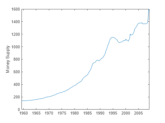
plot(DataTimeTable.Time,DataTimeTable.CPIAUCSL)
ylabel("CPI");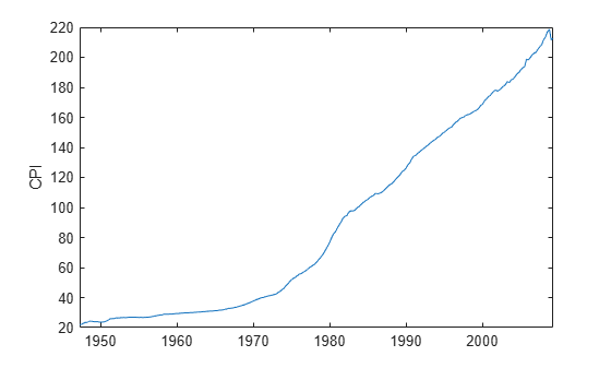
plot(DataTimeTable.Time,DataTimeTable.GDP)
ylabel("GDP")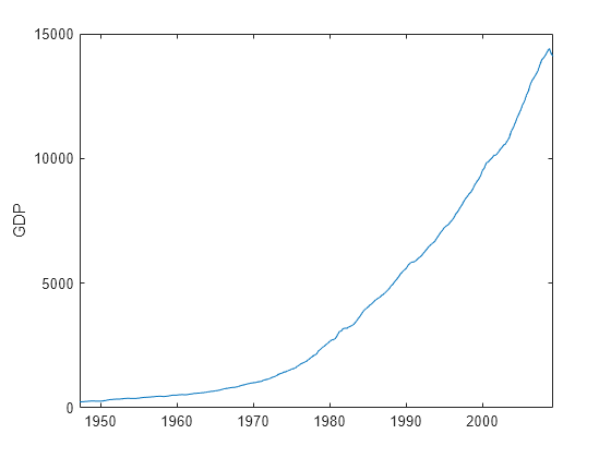
All series are nonstationary.
Stabilize the series.
Convert the M1 money supply prices to returns.
Convert the CPI to the inflation rate.
Convert the GDP to the real GDP rate with respect to year 2000 dollars.
m1slrate = price2ret(DataTimeTable.M1SL);
inflation = price2ret(DataTimeTable.CPIAUCSL);
rgdprate = price2ret(DataTimeTable.GDP./DataTimeTable.GDPDEF);
Preprocess the data by removing all missing observations (indicated by NaN).
tbl = table(m1slrate,inflation,rgdprate);
tbl = rmmissing(tbl);
T = size(tbl,1); % Total sample size
Fit VAR models, with lags ranging from 1 to 4, to the series. Initialize each fit by specifying the first four observations. Store the Akaike information criteria (AIC) of the fits.
numseries = 3;
numlags = (1:4)';
nummdls = numel(numlags);

% Partition time base.
maxp = max(numlags); % Maximum number of required presample responses
idxpre = 1:maxp;
idxest = (maxp + 1):T;

% Preallocation
EstMdl(nummdls) = varm(numseries,0);
aic = zeros(nummdls,1);

% Fit VAR models to data.
Y0 = tbl{idxpre,:}; % Presample
Y = tbl{idxest,:};  % Estimation sample
for j = 1:numel(numlags)
    Mdl = varm(numseries,numlags(j));
    Mdl.SeriesNames = tbl.Properties.VariableNames;
    EstMdl(j) = estimate(Mdl,Y,'Y0',Y0);
    results = summarize(EstMdl(j));
    aic(j) = results.AIC;
end

[~,bestidx] = min(aic);
p = numlags(bestidx)
p =
3
BestMdl = EstMdl(bestidx);
A VAR(3) model yields the best fit.
For each variable and equation in the system, conduct a leave-one-out Granger causality test to assess whether a variable in the fitted VAR(3) model is the 1-step Granger-cause of another variable, given the third variable.
h = gctest(BestMdl)
                          H0                                Decision         Distribution    Statistic     PValue      CriticalValue
    _______________________________________________    __________________    ____________    _________    _________    _____________

    "Exclude lagged inflation in m1slrate equation"    "Cannot reject H0"     "Chi2(3)"       7.0674       0.069782       7.8147
    "Exclude lagged rgdprate in m1slrate equation"     "Cannot reject H0"     "Chi2(3)"       2.5585         0.4648       7.8147
    "Exclude lagged m1slrate in inflation equation"    "Cannot reject H0"     "Chi2(3)"       2.7025         0.4398       7.8147
    "Exclude lagged rgdprate in inflation equation"    "Reject H0"            "Chi2(3)"       14.338      0.0024796       7.8147
    "Exclude lagged m1slrate in rgdprate equation"     "Cannot reject H0"     "Chi2(3)"       7.0352       0.070785       7.8147
    "Exclude lagged inflation in rgdprate equation"    "Reject H0"            "Chi2(3)"       12.006      0.0073619       7.8147
h = 6×1 logical array

   0
   0
   0
   1
   0
   1
gctest conducts six tests, so h is a 6-by-1 logical vector of test decisions corresponding to the rows of the test summary table. The results indicate the following decisions, at a 5% level of significance:
Do not reject the claim that the inflation rate is not the 1-step Granger-cause of the M1 money supply rate, given the real GDP rate (
h(1)=0).Do not reject the claim that the real GDP rate is not the 1-step Granger-cause of the M1 money supply rate, given the inflation rate (
h(2)=0).Do not reject the claim that the M1 money supply rate is not the 1-step Granger-cause of the inflation rate, given the real GDP rate (
h(3)=0).Reject the claim that the real GDP rate is not the 1-step Granger-cause of the inflation rate, given the M1 money supply rate (
h(4)= 1).Do not reject the claim that the M1 money supply rate is not the 1-step Granger-cause of the real GDP rate, given the inflation rate (
h(5)=0).Reject the claim that the inflation rate is not the 1-step Granger-cause of the real GDP rate, given the M1 money supply rate (
h(6)= 1).
Because the inflation and real GDP rates are 1-step Granger-causes of each other, they constitute a feedback loop.
Consider the 3-D VAR(3) model and leave-one-out Granger causality test in Conduct Leave-One-Out Granger Causality Test.
Load the US macroeconomic data set Data_USEconModel.mat. Preprocess the data. Fit a VAR(3) model to the preprocessed data.
load Data_USEconModel

m1slrate = price2ret(DataTimeTable.M1SL);
inflation = price2ret(DataTimeTable.CPIAUCSL);
rgdprate = price2ret(DataTimeTable.GDP./DataTimeTable.GDPDEF);

tbl = table(m1slrate,inflation,rgdprate);
tbl = rmmissing(tbl);

Mdl = varm(3,3);
Mdl.SeriesNames = tbl.Properties.VariableNames;
EstMdl = estimate(Mdl,tbl{5:end,:},'Y0',tbl{2:4,:});
Conduct an exclude-all Granger causality test on the variables of the fitted model.
h = gctest(EstMdl,'Type',"exclude-all");
                               H0                                    Decision         Distribution    Statistic     PValue      CriticalValue
    ________________________________________________________    __________________    ____________    _________    _________    _____________

    "Exclude all but lagged m1slrate in m1slrate equation"      "Cannot reject H0"     "Chi2(6)"        9.477        0.14847       12.592
    "Exclude all but lagged inflation in inflation equation"    "Reject H0"            "Chi2(6)"       19.475      0.0034327       12.592
    "Exclude all but lagged rgdprate in rgdprate equation"      "Reject H0"            "Chi2(6)"        19.16      0.0039014       12.592
gctest conducts numtests = 3 tests. The results indicate the following decisions, each at a 5% level of significance:
Do not reject the claim that the inflation and real GDP rates do not Granger-cause the M1 money supply rate.
Reject the claim that the M1 money supply and real GDP rates do not Granger-cause the inflation rate.
Reject the claim that the M1 money supply and inflation rates do not Granger-cause the real GDP rate.
The false discovery rate increases with the number of simultaneous hypothesis tests you conduct. To combat the increase, decrease the level of significance per test by using the 'Alpha' name-value pair argument. Consider the 3-D VAR(3) model and leave-one-out Granger causality test in Conduct Leave-One-Out Granger Causality Test.
Load the US macroeconomic data set Data_USEconModel.mat. Preprocess the data. Fit a VAR(3) model to the preprocessed data.
load Data_USEconModel

m1slrate = price2ret(DataTimeTable.M1SL);
inflation = price2ret(DataTimeTable.CPIAUCSL);
rgdprate = price2ret(DataTimeTable.GDP./DataTimeTable.GDPDEF);
tbl = table(m1slrate,inflation,rgdprate);
tbl = rmmissing(tbl);

Mdl = varm(3,3);
Mdl.SeriesNames = tbl.Properties.VariableNames;
EstMdl = estimate(Mdl,tbl{5:end,:},'Y0',tbl{2:4,:});
A leave-one-out Granger causality test on the variables in the model results in numtests = 6 simultaneous tests. Conduct the tests, but specify a family-wise significance level of 0.05 by specifying a level of significance of alpha = 0.05/numtests for each test.
numtests = 6;
alpha = 0.05/numtests
alpha =
0.0083
gctest(EstMdl,'Alpha',alpha); H0 Decision Distribution Statistic PValue CriticalValue
_______________________________________________ __________________ ____________ _________ _________ _____________
"Exclude lagged inflation in m1slrate equation" "Cannot reject H0" "Chi2(3)" 7.0674 0.069782 11.739
"Exclude lagged rgdprate in m1slrate equation" "Cannot reject H0" "Chi2(3)" 2.5585 0.4648 11.739
"Exclude lagged m1slrate in inflation equation" "Cannot reject H0" "Chi2(3)" 2.7025 0.4398 11.739
"Exclude lagged rgdprate in inflation equation" "Reject H0" "Chi2(3)" 14.338 0.0024796 11.739
"Exclude lagged m1slrate in rgdprate equation" "Cannot reject H0" "Chi2(3)" 7.0352 0.070785 11.739
"Exclude lagged inflation in rgdprate equation" "Reject H0" "Chi2(3)" 12.006 0.0073619 11.739
The test decisions of these more conservative tests are the same as the tests decisions in Conduct Leave-One-Out Granger Causality Test. However, the conclusions of the conservative tests hold simultaneously at a 5% level of significance.
Consider the 3-D VAR(3) model and leave-one-out Granger causality test in Conduct Leave-One-Out Granger Causality Test.
Load the US macroeconomic data set Data_USEconModel.mat. Preprocess the data. Fit a VAR(3) model to the preprocessed data.
load Data_USEconModel

m1slrate = price2ret(DataTimeTable.M1SL);
inflation = price2ret(DataTimeTable.CPIAUCSL);
rgdprate = price2ret(DataTimeTable.GDP./DataTimeTable.GDPDEF);

tbl = table(m1slrate,inflation,rgdprate);
tbl = rmmissing(tbl);

Mdl = varm(3,3);
Mdl.SeriesNames = tbl.Properties.VariableNames;
EstMdl = estimate(Mdl,tbl{5:end,:},'Y0',tbl{2:4,:});
Conduct a leave-one-out Granger causality test on the variables of the fitted model. Return the test result summary table and suppress the test results display.
[~,Summary] = gctest(EstMdl,'Display',false)Summary=6×6 table
H0 Decision Distribution Statistic PValue CriticalValue
_______________________________________________ __________________ ____________ _________ _________ _____________
"Exclude lagged inflation in m1slrate equation" "Cannot reject H0" "Chi2(3)" 7.0674 0.069782 7.8147
"Exclude lagged rgdprate in m1slrate equation" "Cannot reject H0" "Chi2(3)" 2.5585 0.4648 7.8147
"Exclude lagged m1slrate in inflation equation" "Cannot reject H0" "Chi2(3)" 2.7025 0.4398 7.8147
"Exclude lagged rgdprate in inflation equation" "Reject H0" "Chi2(3)" 14.338 0.0024796 7.8147
"Exclude lagged m1slrate in rgdprate equation" "Cannot reject H0" "Chi2(3)" 7.0352 0.070785 7.8147
"Exclude lagged inflation in rgdprate equation" "Reject H0" "Chi2(3)" 12.006 0.0073619 7.8147
Summary is a MATLAB table containing numtests = 6 rows. The rows contain the results of each test. The columns are table variables containing characteristics of the tests.
Extract the -values of the tests.
pvalues = Summary.PValue
pvalues = 6×1

    0.0698
    0.4648
    0.4398
    0.0025
    0.0708
    0.0074
Time series are block exogenous if they do not Granger-cause any other variables in a multivariate system. Test whether the effective federal funds rate is block exogenous with respect to the real GDP, personal consumption expenditures, and inflation rates.
Load the US macroeconomic data set Data_USEconModel.mat. Convert the price series to returns.
load Data_USEconModel
inflation = price2ret(DataTimeTable.CPIAUCSL);
rgdprate = price2ret(DataTimeTable.GDP./DataTimeTable.GDPDEF);
pcerate = price2ret(DataTimeTable.PCEC);
Test whether the federal funds rate is nonstationary by conducting an augmented Dickey-Fuller test. Specify that the alternative model has a drift term and an test.
StatTbl = adftest(DataTimeTable,DataVariable="FEDFUNDS",Model="ard")
StatTbl=1×8 table
                h       pValue      stat      cValue     Lags    Alpha     Model      Test
              _____    ________    _______    _______    ____    _____    _______    ______

    Test 1    false    0.071419    -2.7257    -2.8751     0      0.05     {'ARD'}    {'T1'}
The test decision h = 0 indicates that the null hypothesis that the series has a unit root should not be rejected, at 0.05 significance level.
To stabilize the federal funds rate series, apply the first difference to it.
dfedfunds = diff(DataTimeTable.FEDFUNDS);
Preprocess the data by removing all missing observations (indicated by NaN).
tbl = table(inflation,pcerate,rgdprate,dfedfunds);
tbl = rmmissing(tbl);
T = size(tbl,1); % Total sample size
Assume a 4-D VAR(3) model for the four series. Initialize the model by using the first three observations, and fit the model to the rest of the data. Assign names to the series in the model.
Mdl = varm(4,3);
Mdl.SeriesNames = tbl.Properties.VariableNames;
EstMdl = estimate(Mdl,tbl{4:end,:},Y0=tbl{1:3,:});
Assess whether the federal funds rate is block exogenous with respect to the real GDP, personal consumption expenditures, and inflation rates. Conduct an -based Wald test, and return the test decision and summary table. Suppress the test results display.
cause = "dfedfunds";
effects = ["inflation" "pcerate" "rgdprate"];
[h,Summary] = gctest(EstMdl,Type="blockwise", ...
    Cause=cause,Effect=effects,Test="f",Display=false);
gctest conducts one test. h = 1 indicates, at a 5% level of significance, rejection of the null hypothesis that the federal funds rate is block exogenous with respect to the other variables in the VAR model. This result suggests that the federal funds rate Granger-causes at least one of the other variables in the system.
Alternatively, you can conduct the same blockwise Granger causality test by passing the data to the gctest function.
causedata = tbl.dfedfunds;
EffectsData = tbl{:,effects};
[hgc,pvalue,stat,cvalue] = gctest(causedata,EffectsData,...
    NumLags=3,Test="f")
hgc = logical
1
pvalue =
9.0805e-09
stat =
6.9869
cvalue =
1.9265
To determine which variables are Granger-caused by the federal funds rate, conduct a leave-one-out test and specify the "cause" and "effects."
gctest(EstMdl,Cause=cause,Effect=effects);
                           H0                            Decision      Distribution    Statistic      PValue      CriticalValue
    ________________________________________________    ___________    ____________    _________    __________    _____________

    "Exclude lagged dfedfunds in inflation equation"    "Reject H0"     "Chi2(3)"       26.157      8.8433e-06       7.8147
    "Exclude lagged dfedfunds in pcerate equation"      "Reject H0"     "Chi2(3)"       10.151        0.017325       7.8147
    "Exclude lagged dfedfunds in rgdprate equation"     "Reject H0"     "Chi2(3)"       10.651        0.013772       7.8147
The test results suggest the following decisions, each at a 5% level of significance:
Reject the claim that the federal funds rate is not a 1-step Granger-cause of the inflation rate, given all other variables in the VAR model.
Reject the claim that the federal funds rate is not a 1-step Granger-cause of the personal consumption expenditures rate, given all other variables in the VAR model.
Reject the claim that the federal funds rate is not a 1-step Granger-cause of the real GDP rate, given all other variables in the VAR model.
Input Arguments
Name-Value Arguments
Output Arguments
More About
Tips
gctestuses the series names inMdlin test result summaries. To make the output more meaningful for your application, specify series names by setting theSeriesNamesproperty of the VAR model objectMdlby using dot notation before callinggctest. For example, the following code assigns names to the variables in the 3-D VAR model objectMdl:Mdl.SeriesNames = ["rGDP" "m1sl" "inflation"];
The exclude-all and leave-one-out Granger causality tests conduct multiple, simultaneous tests. To control the inevitable increase in the false discovery rate, decrease the level of significance
Alphawhen you conduct multiple tests. For example, to achieve a family-wise significance level of 0.05, specify'Alpha',0.05/numtests.
Algorithms
The name-value pair arguments Cause and Effect
apply to the block-wise Granger causality test because they specify which equations have lag
coefficients set to 0 for the null hypothesis. Because the leave-one-out and exclude-all
Granger causality tests cycle through all combinations of variables in the VAR model, the
information provided by Cause and Effect is not
necessary. However, you can specify a leave-one-out or exclude-all Granger causality test and
the Cause and Effect variables to conduct unusual
tests such as constraints on self lags. For example, the following code assesses the null
hypothesis that the first variable in the VAR model Mdl is not the 1-step
Granger-cause of
itself:
gctest(Mdl,'Type',"leave-one-out",'Cause',1,'Effect',1);
References
[1] Granger, C. W. J. "Investigating Causal Relations by Econometric Models and Cross-Spectral Methods." Econometrica. Vol. 37, 1969, pp. 424–459.
[2] Hamilton, James D. Time Series Analysis. Princeton, NJ: Princeton University Press, 1994.
[3] Dolado, J. J., and H. Lütkepohl. "Making Wald Tests Work for Cointegrated VAR Systems." Econometric Reviews. Vol. 15, 1996, pp. 369–386.
[4] Lütkepohl, Helmut. New Introduction to Multiple Time Series Analysis. New York, NY: Springer-Verlag, 2007.
[5] Toda, H. Y., and T. Yamamoto. "Statistical Inferences in Vector Autoregressions with Possibly Integrated Processes." Journal of Econometrics. Vol. 66, 1995, pp. 225–250.