covarianceDenoising
Syntax
Description
SigmaHat = covarianceDenoising(AssetReturns)
In addition, you can use covarianceShrinkage to compute an estimate of covariance matrix
using shrinkage estimation. For information on which covariance estimation method to
choose, see Comparison of Methods for Covariance Estimation.
SigmaHat = covarianceDenoising(Sigma,SampleSize)Sigma) and the sample size used to estimate the initial
covariance (sampleSize).
[
returns a covariance estimate and the number of eigenvalues that are associated with
signal in combination with either of the input argument combinations in the previous
syntaxes.SigmaHat,numSignalEig] = covarianceDenoising(___)
Examples
This example shows how to use covariance denoising to reduce noise and enhance the signal of the empirical covariance matrix. In mean-variance portfolio optimization, a noisy estimate of the covariance estimate results in unstable solutions that cause high turnover and transaction costs. Ideally, to decrease the estimation error, it is desirable to increase the sample size. Yet, there are cases where this is not possible. In extreme cases in which the number of assets is larger than the number of observations, the traditional covariance matrix results in a singular matrix. Working with a nearly singular or an ill-conditioned covariance matrix magnifies the impact of estimation errors.
Compute a portfolio efficient frontier using different covariance estimates with the same sample data.
% Load portfolio data with 225 assets
load port5.mat
covariance = corr2cov(stdDev_return,Correlation);
% Generate a sample with 200 observations
rng('default')
nScen = 200;
retSeries = portsim(mean_return',covariance,nScen);
Compute the traditional and denoised covariance estimates. Use covarianceDenoising to create a covariance estimate.
Sigma = cov(retSeries);
denoisedSigma = covarianceDenoising(retSeries);
Compute the condition number of both covariance estimates. The denoised covariance denoisedSigma has a lower condition number than the traditional covariance estimate Sigma.
conditionNum = [cond(Sigma); cond(denoisedSigma)];
condNumT = table(conditionNum,'RowNames',{'Sigma','SigmaHat'})
condNumT=2×1 table
                conditionNum
                ____________

    Sigma        6.8746e+18
    SigmaHat         1046.8
Use Portfolio to construct Portfolio objects that use the different AssetCovar values. Then use setDefaultConstraints to set the portfolio constraints with nonnegative weights that sum to 1 for the three portfolios: the true mean with the true covariance, the traditional covariance estimate, and the denoised estimate.
% Create a Portfolio object with the true parameters
p = Portfolio(AssetMean=mean_return,AssetCovar=covariance);
p = setDefaultConstraints(p);

% Create a Portfolio object with true mean and traditional covariance estimate
pTraditional = Portfolio(AssetMean=mean_return,AssetCovar=Sigma);
pTraditional = setDefaultConstraints(pTraditional);

% Create a Portfolio object with true mean and denoised covariance
pDenoised = Portfolio(AssetMean=mean_return,AssetCovar=denoisedSigma);
pDenoised = setDefaultConstraints(pDenoised);
Use estimateFrontier to estimate the efficient frontier for each of the Portfolio objects.
% Number of portfolios on the efficient frontier
nPort = 20;

% True efficient portfolios
w = estimateFrontier(p,nPort);

% Traditional covariance efficient portfolios
wTraditional = estimateFrontier(pTraditional,nPort);

% Denoised covariance efficient portfolios
wDenoised = estimateFrontier(pDenoised,nPort);
Use plotFrontier to plot the frontier obtained from the different weights using the true parameter values.
figure
plotFrontier(p,w)
hold on
plotFrontier(p,wTraditional)
plotFrontier(p,wDenoised)
legend('True frontier','Traditional frontier','Denoised frontier', ...
    Location='southeast');
hold off

The efficient frontier obtained by denoising is closer to the true frontier than the frontier obtained using the traditional covariance estimate. This improvement shows the robustness of the denoised covariance estimate.
This example shows the effect of the sample size in covarianceDenoising to compute a denoised version of an initial covariance estimate. The covarianceDenoising function has two different syntaxes. This example focuses on the syntax with two inputs: a covariance estimate and the size of the sample that you use to compute the initial covariance estimate. This example demonstrates an empirical study of the effect of the sample size on the accuracy of the denoised estimate. The goal of this example is to provide insight for the choice of the sample size when this information is not available. This scenario can happen if the initial covariance estimate is stored but the information of the sample used to compute the estimate is not available.
Create Random Sample
Create a random sample using mvnrnd.
% Load data
load('port5.mat','mean_return','Correlation')

% Select the number of assets
numObservations = 300;
numAssets = 100;
mu = mean_return(1:numAssets);
C = Correlation(1:numAssets,1:numAssets);

% Generate a random sample
rng('default')
randSample = mvnrnd(mu,C,numObservations);
Use corr to compute the standard correlation estimate of the sample. This example works with the correlation matrix to remove the effect of the variance. This is useful when comparing the effect of the sample size in the denoised covariance estimate.
stdCorr = corr(randSample);
Due to numerical errors, stdCorr is not symmetric. Modify stdCorr to make it symmetric.
% Compute maximum absolute difference of matrix against its
% transpose
max(abs(stdCorr-stdCorr'),[],'all')
ans =
0
% Force correlation matrix to be symmetric
stdCorr = (stdCorr+stdCorr')/2;
Use covarianceDenoising to compute the denoised covariance estimate from Sigma using the correct sample size.
denoisedCorr = covarianceDenoising(stdCorr,numObservations);
denoisedCorr = (denoisedCorr+denoisedCorr')/2;
Compute Denoised Covariance for Different Sample Sizes
Compare the maximum correlation difference between the denoised covariance with the correct sample size and other sample sizes. Also, you compute the number of factors.
% Sample sizes to try
numSizes = 100;
sampleSizes = ceil(logspace(0,4,numSizes));

% Compute denoised correlation and store the maximum correlation
% mismatch
correlations = cell(numSizes);
numFactors = zeros(numSizes,1);
maxDiff = zeros(numSizes,1);
for i = 1:numSizes
    [correlations{i},numFactors(i)] = covarianceDenoising(stdCorr,...
        sampleSizes(i));
    maxDiff(i) = norm(correlations{i}(:)-denoisedCorr(:),inf);
end
Plot the maximum error in the correlations as well as the number of factors identified for each sample size.
figure;

% Plot correlation error
yyaxis left
semilogx(sampleSizes,maxDiff)
hold on
ylabel("Correlation Error");

% Plot number of factors
yyaxis right
semilogx(sampleSizes,numFactors)
ylabel("Number of Factors");

% Title, labels, and legends
title("Sample Size Effect")
xlabel("Sample Size");
hold off
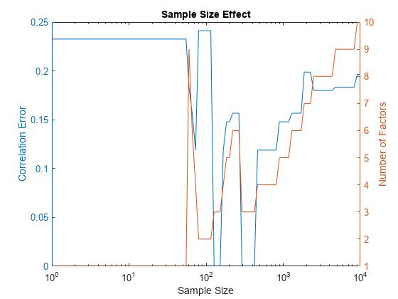
Note that when the sample size is close to the number of assets, the behavior of both the correlation error and the number of factors is erratic. Here, when the sample size is between 55 and 292, the number of factors and the correlation error jump up and down. Before 55 "observations" the number of factors is 1 because the denoising method doesn't have enough information to trust that what is being observed is signal and not noise; only the largest eigenvalue is associated with signal. Usually the largest eigenvalue is linked to the market. Meanwhile, after 292 "observations" the number of eigenvalues not associated with noise monotonically increases. This behavior happens because denoising assumes that the sample is less noisy with more observations, so identifying signal from noise is easier.
If the sample size of the initial covariance estimate is not known, it is better to choose a sample size that is far from the number of assets. For cases with less trust in the initial covariance estimate, the sample size should be smaller, below 55 in this example. If you trust the initial covariance estimate, then the sample size should be larger, above 292 in this example. The degree of trust in the initial covariance matrix can be adjusted by increasing the sample size.
This example compares a minimum variance investment strategy using the traditional covariance estimate with a minimum variance strategy using covariance denoising.
Load Data
% Read a table of daily adjusted close prices for 2006 DJIA stocks.
T = readtable('dowPortfolio.xlsx');

% Convert the table to a timetable.
pricesTT = table2timetable(T,'RowTimes','Dates');
numAssets = size(pricesTT.Variables, 2);
Use the first 42 days of the dowPortfolio.xlsx data set to initialize the backtest strategies. The backtest is then run over the remaining data.
warmupPeriod = 42;
Compute Initial Weights
Use the traditionalStrat and denoisedStrat functions in Local Functions to compute the weights.
% Specify no current weights (100% cash position).
w0 = zeros(1,numAssets);

% Specify warm-up partition of data set timetable.
warmupTT = pricesTT(1:warmupPeriod,:);

% Compute the initial portfolio weights for each strategy.
traditional_initial = traditionalStrat(w0,warmupTT);
shrunk_initial = denoisedStrat(w0,warmupTT);
Create Backtest Strategies
Create Traditional and Denoising backtest strategy objects using backtestStrategy.
% Rebalance approximately every month.
rebalFreq = 21;

% Set the rolling lookback window to be at least 2 months and at
% most 6 months.
lookback  = [42 126];

% Use a fixed transaction cost (buy and sell costs are both 0.5%
% of amount traded).
transactionsFixed = 0.005;

% Specify the strategy objects.
strat1 = backtestStrategy('Traditional', @traditionalStrat, ...
    RebalanceFrequency=rebalFreq, ...
    LookbackWindow=lookback, ...
    TransactionCosts=transactionsFixed, ...
    InitialWeights=traditional_initial);

strat2 = backtestStrategy('Denoising', @denoisedStrat, ...
    RebalanceFrequency=rebalFreq, ...
    LookbackWindow=lookback, ...
    TransactionCosts=transactionsFixed, ...
    InitialWeights=shrunk_initial);

% Aggregate the two strategy objects into an array.
strategies = [strat1, strat2];
Create a backtestEngine object then use runBacktest to run the backtest.
% Create the backtesting engine object.
backtester = backtestEngine(strategies);

% Run the backtest.
backtester = runBacktest(backtester,pricesTT,'Start',warmupPeriod);

% Generate summary table of the performance of the strategies.
summary(backtester)
ans=9×2 table
                       Traditional    Denoising
                       ___________    __________

    TotalReturn           0.13432        0.12745
    SharpeRatio           0.10807        0.10719
    Volatility          0.0057472      0.0055101
    AverageTurnover     0.0098376      0.0074213
    MaxTurnover           0.36237         0.2791
    AverageReturn      0.00061961     0.00058922
    MaxDrawdown          0.058469       0.053624
    AverageBuyCost        0.51635        0.38982
    AverageSellCost       0.51635        0.38982
Compare Performance of Strategies
Use equityCurve to plot the equity curve to compare the performance of both strategies.
equityCurve(backtester)

The maximum and average turnover are decreased using covariance denoising. Also, the covariance denoising strategy results in a decrease of buy and sell costs. In this example, not only is the turnover decreased, but also the volatility and the maximum drawdown are decreased. Therefore, in this example the denoised covariance produces more robust weights.
Local Functions
function new_weights = traditionalStrat(~, pricesTT)
% Function for minimum variance portfolio using traditional covariance estimate.

% Compute the returns from the prices timetable.
assetReturns = tick2ret(pricesTT);
mu = mean(assetReturns.Variables);
Sigma = cov(assetReturns.Variables,"omitrows");

% Create the portfolio problem.
p = Portfolio(AssetMean=mu,AssetCovar=Sigma);
% Specify long-only fully invested contraints.
p = setDefaultConstraints(p);

% Compute the minimum variance portfolio.
new_weights = estimateFrontierLimits(p,'min');
end

function new_weights = denoisedStrat(~, pricesTT)
% Function for minimum variance portfolio using covariance denoising.

% Compute the returns from the prices timetable.
assetReturns = tick2ret(pricesTT);
mu = mean(assetReturns.Variables);
Sigma = covarianceDenoising(assetReturns.Variables);

% Create the portfolio problem.
p = Portfolio(AssetMean=mu,AssetCovar=Sigma);
% Specify long-only fully invested contraints.
p = setDefaultConstraints(p);

% Compute the minimum variance portfolio.
new_weights = estimateFrontierLimits(p,'min');
end
Input Arguments
Output Arguments
More About
Algorithms
The covarianceDenoising function shrinks only the part of the
covariance that corresponds with noise as follows:
Compute the correlation matrix C associated with the traditional covariance estimate Σ.
Compute the eigendecomposition of C = VΛ VT.
Estimate the empirical distribution of the eigenvalues using kernel density estimation with
fitdist(x,'Kernel'). For more information, seefitdist.Fit the Marchenko-Pastur distribution to the empirical distribution by minimizing the mean squared error (MSE) between the empirical probability density function (pdf) and the fitted Marchenko-Pastur pdf. This gives the theoretical bounds λ+ and λ- on the eigenvalues associated with noise.
Let be the average of the eigenvalues smaller than λ+. Set all eigenvalues smaller than λ+ to . These are the eigenvalues associated with noise.
Compute the denoised version of the correlation matrix and rescale so that the main diagonal only has ones. is a correlation matrix.
Compute the denoised covariance estimate from .
References
[1] Lòpez de Prado, M. Machine Learning for Asset Managers (Elements in Quantitative Finance). Cambridge University Press, 2020.
Version History
Introduced in R2023a