Estimate Process Model
Estimate continuous-time process model for single-input, single-output (SISO) system in either time or frequency domain in the Live Editor
Description
The Estimate Process Model task lets you interactively estimate and validate a process model for SISO systems. You can define and vary the model structure and specify optional parameters, such as initial condition handling and search methods. The task automatically generates MATLAB® code for your live script. For more information about Live Editor tasks generally, see Add Interactive Tasks to a Live Script.
Process models are simple continuous-time transfer functions that describe the linear system dynamics. Process model elements include static gain, time constants, time delays, integrator, and process zero.
Process models are popular for describing system dynamics in numerous industries and are applicable to various production environments. The advantages of these models are that they are simple, they support transport delay estimation, and the model coefficients are easy to interpret as poles and zeros. For more information about process model estimation, see What Is a Process Model?
The Estimate Process Model task is independent of the more general System Identification app. Use the System Identification app when you want to compute and compare estimates for multiple model structures.
To get started, load experiment data that contains input and output data into your MATLAB workspace and then import that data into the task. Then select a model structure to estimate. The task gives you controls and plots that help you experiment with different model structures and compare how well the output of each model fits the measurements.
Open the Task
To add the Estimate Process Model task to a live script in the MATLAB Editor:
On the Live Editor tab, select Task > Estimate Process Model.
In a code block in your script, type a relevant keyword, such as
processorestimate. SelectEstimate Process Modelfrom the suggested command completions.
Examples
Use the Estimate Process Model Live Editor Task to estimate a process model and compare the model output to the measurement data.
Set Up Data
Load the measurement data tt1 into your MATLAB workspace. tt1 is a timetable that contains one input variable u and one output variable y.
load sdata1 tt1
Import Data into the Task
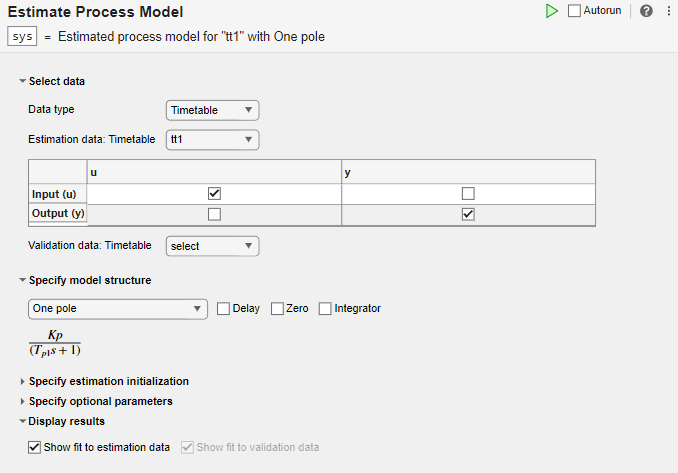
In the Select data section, set Data type to Timetable and set Estimation data to tt1.
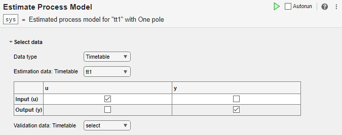
The task displays a table that contains the tt1 input and output variable names.
Estimate the Model Using Default Settings
Examine the model structure and optional parameters.
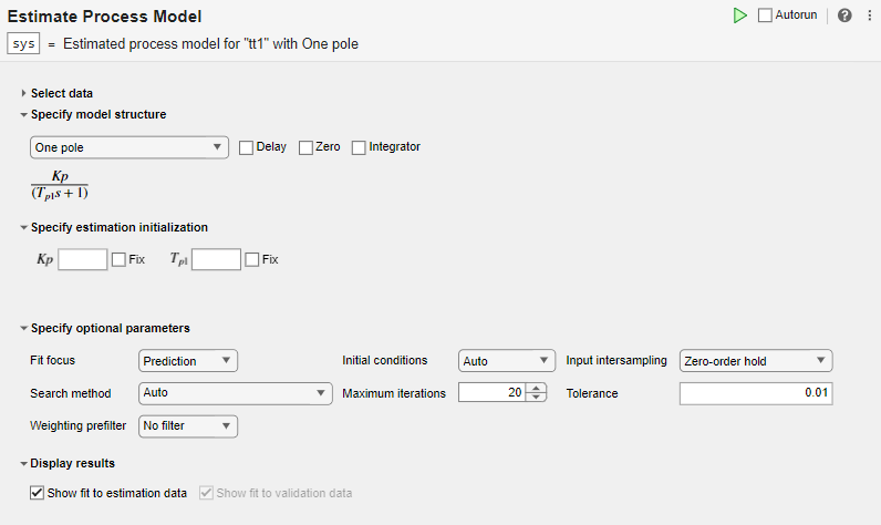
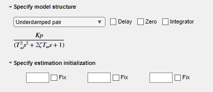
In the Specify model structure section, the default option is One Pole with no delay, zero, or integrator. Equations below the parameters in this section display the specified structure.
In the Specify estimation initialization section, initialization parameters matching the parameters in your model structure allow you to set starting points for estimation. If you select Fix, the parameter remains fixed to the value you specify. For this example, do not specify initialization. The task then uses default values for starting points.
In the Specify optional parameters section, the default options for process estimation are set.
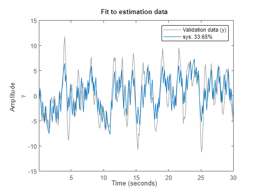
Execute the task from the Live Editor tab by clicking the green arrow. You can also select Autorun to run the task automatically every time you update a parameter.
![]()
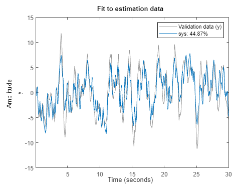
A plot displays the estimation data, the estimated model output, and the fit percentage.
Experiment with Parameter Settings
Experiment with the parameter settings and see how they influence the fit.
For instance, add delay to the One Pole structure and run the task.

The estimation fit improves, although the fit percentage is still below 50%.
Try a different model structure. In Specify model structure, select Underdamped Pair with no delay and run the task.

The fit results improve significantly.
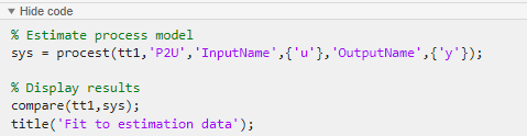
Generate Code
To display the code that the task generates, click ![]() at the bottom of the parameter section. The code that you see reflects the current parameter configuration of the task.
at the bottom of the parameter section. The code that you see reflects the current parameter configuration of the task.
Use separate estimation and validation data so that you can validate the estimated process model.
Set Up Data
Load the measurement data sdata1 into your MATLAB workspace and examine its contents.
load sdata1 umat1 ymat1 Ts
Split the data into two sets, with one half for estimation and one half for validation. The original data set has 300 samples, so each new data set has 150 samples.
u_est = umat1(1:150);
u_val = umat1(151:300);
y_est = ymat1(1:150);
y_val = ymat1(151:300);
Ts
Ts =
0.1000
Import Data into Task
In the Select data section, set Data type to Numeric. Set the sample time to 0.1 seconds. Select the appropriate data sets for estimation and validation.

Estimate and Validate the Model
The example Estimate Process Model with Live Editor Task achieves the best results using the model structure Underdamped Pair. Choose the same option for this example.

Execute the task. Executing the task creates two plots. The first plot shows the estimation results and the second plot shows the validation results.

The fit to the estimation data is somewhat worse than in Estimate Process Model with Live Editor Task. Estimation in the current example has only half the data with which to estimate the model. The fit to the validation data, which represents the goodness of the model more generally, is better than the fit to the estimation data.